The matrix language is the core of the numerical part of Euler. It allows generating tables of functions without the need to write loops.
Of course, it can also be used to compute expressions with vectors and matrices. That part of EMT is explained in detail in the tutorial on linear algebra.
Introduction to Linear Algebra
First of all, a matrix can be defined element by element. Separate the elements with ",", and the rows with ";".
Let us enter a 3x3 matrix and assign it to the variable A. For this notebook, we switch to a short format for the output of Euler.
>shortformat; A=[1,2,3;4,5,6;7,8,9]
        1         2         3
        4         5         6
        7         8         9
Incomplete rows will be filled with 0.
>[1,2,3;3,4]
        1         2         3
        3         4         0
A matrix with one row is a row vector. The matrix language makes a difference between row and column vectors.
>v=[1,2,3]
[1, 2, 3]
The : operator creates equal spaced vectors. By default the increment is 1.
>1:3
[1, 2, 3]
But the increment can also be any other value.
>1:0.2:2
[1, 1.2, 1.4, 1.6, 1.8, 2]
Even negative.
>10:-1:1
[10, 9, 8, 7, 6, 5, 4, 3, 2, 1]
For a narrower output use shortformat, shortestformat, or fracformat. In the following command, we use four places for the output with no decimal fraction. The function intrandom generates integer random numbers.
>format(4,0); intrandom(10,10,6), shortformat;
  2   2   4   5   5   2   2   5   6   5
  4   3   1   4   5   4   5   1   6   1
  6   5   1   2   6   3   6   1   4   2
  1   5   4   4   6   6   1   5   2   6
  1   6   6   4   4   5   2   6   3   3
  3   5   1   2   3   5   2   2   1   6
  3   6   3   1   2   3   2   5   5   4
  2   2   3   1   2   3   4   6   4   6
  1   4   1   4   3   2   5   5   5   4
  1   6   6   3   2   1   1   3   5   3
For a column vector, use a 1xn matrix.
>[1;2;3]
        1
        2
        3
Or transpose a row vector.
>[1,2,3]'
        1
        2
        3
The basic rule of the matrix language is:
"All operators and functions are applied element for element to the matrix or vector."
Thus the following is simply a vector of products of the elements of a vector v with the elements of a vector w.
>v=[1,2,3]; w=[2,3,4]; v*w
[2, 6, 12]
Since v was 1,2,3, and v*v multiplies each element of v with itself, we get all elements squared. So the result w has the property
![]()
Note that this is different from the matrix product or the inner product!
Other operators work in the same way. So v^2 will be the vector of elements of v squared.
>v^2
[1, 4, 9]
It also works the other way around.
>2^v
[2, 4, 8]
Or like this.
>v^v
[1, 4, 27]
Not only operators, but almost all mathematical functions are applied element for element to a matrix or vector.
>sqrt(v)
[1, 1.41421, 1.73205]
This also applies to matrices.
>A = [1,2,3;4,5,6;7,8,9]
        1         2         3
        4         5         6
        7         8         9
Always remember that * is not the matrix product.
>A*A
        1         4         9
       16        25        36
       49        64        81
The matrix product uses the "." operator.
>A.A
       30        36        42
       66        81        96
      102       126       150
If one of the operands is a vector or a scalar it is expanded in the natural way.
>2*A
        2         4         6
        8        10        12
       14        16        18
E.g., if the operand is a column vector its elements are applied to all rows of A.
>[1;2;3]*A
        1         2         3
        8        10        12
       21        24        27
If it is a row vector it is applied to all columns of A.
>A*[1,2,3]
        1         4         9
        4        10        18
        7        16        27
One can imagine this multiplication as if the row vector v had been duplicated to form a matrix of the same size as A.
>A*dup([1,2,3],3)
        1         4         9
        4        10        18
        7        16        27
This does also apply for two vectors where one is a row vector and the other is a column vector.
>(1:5)*(1:5)'
        1         2         3         4         5
        2         4         6         8        10
        3         6         9        12        15
        4         8        12        16        20
        5        10        15        20        25
Again, remember that this is not the matrix product!
>(1:5).(1:5)'
55
Even operators like < or == work in the same way.
>(1:10)<6
[1, 1, 1, 1, 1, 0, 0, 0, 0, 0]
E.g., we can count the number of elements satisfying a certain condition with the function sum().
>sum((1:10)<6)
5
Let us define a smaller matrix.
>B=[1,2;3,4]
        1         2
        3         4
To compute the inverse we have to use the function inv.
>inv(B)
       -2         1
      1.5      -0.5
Let us check the inverse.
>B.inv(B)
        1         0
        0         1
B^(-1) is not the inverse of B! By the mapping rule, it will invert all elements of B.
>B^(-1)
        1       0.5
 0.333333      0.25
As an extension to inv(), there is the function matrixpower().
>matrixpower(B,-1)
       -2         1
      1.5      -0.5
It works for integer exponents.
>matrixpower(B,-3).matrixpower(B,3)
        1         0
        0         1
We can print a matrix using fractional output.
>fraction inv(B);
       -2         1
      3/2      -1/2
Euler is a numerical program. So we do not get the exact inverse. But to see the error, we have to choose a longer format.
>longest B.inv(B)
     0.9999999999999998  1.110223024625157e-016
                      0                       1
Of course, Maxima can be used for such simple linear algebra problems. We can define the matrix for Euler and Maxima with &:=, and then use it in symbolic expressions.
>B &:= [1,2;3,4]; &invert(B)
                             [ - 2   1  ]
                             [          ]
                             [  3     1 ]
                             [  -   - - ]
                             [  2     2 ]
The result can be evaluated numerically in Euler. For more information about Maxima, see the introduction to Maxima.
>&invert(B)()
       -2         1
      1.5      -0.5
Euler has also a powerful function xinv(), which makes a bigger effort and gets more exact results.
Note, that with &:= the matrix B has been defined as symbolic in symbolic expressions and as numerical in numerical expressions. So we can use it here.
>longest B.xinv(B)
                      1                       0
                      0                       1
To transpose a matrix we use the apostrophe.
>v=1:4; v'
        1
        2
        3
        4
So we can compute matrix A times vector b.
>A=[1,2,3,4;5,6,7,8]; A.v'
       30
       70
Note that v is still a row vector. So v'.v is different from v.v'.
>v'.v
        1         2         3         4
        2         4         6         8
        3         6         9        12
        4         8        12        16
v.v' computes the norm of v squared for row vectors v. The result is a 1x1 vector, which works just like a real number.
>v.v'
30
There is also the function norm (along with many other function of Linear Algebra).
>norm(v)^2
30
E.g. the eigenvalues of A can be computed numerically.
>A=[1,2,3;4,5,6;7,8,9]; real(eigenvalues(A))
[16.1168, -1.11684, 0]
Or symbolically. See the tutorial about Maxima for details on this.
>&eigenvalues(@A)
            15 - 3 sqrt(33)  3 sqrt(33) + 15
          [[---------------, ---------------, 0], [1, 1, 1]]
                   2                2
To access a matrix element, use the bracket notation.
>A=[1,2,3;4,5,6;7,8,9], A[2,2]
        1         2         3
        4         5         6
        7         8         9
5
We can access a complete line of a matrix.
>A[2]
[4, 5, 6]
In case of row or column vectors, this returns an element of the vector.
>v=1:3; v[2]
2
To make sure, you get the first row for a 1xn and a mxn matrix, specify all columns using an empty second index.
>A[2,]
[4, 5, 6]
If the index is a vector of indices, Euler will return the corresponding rows of the matrix.
Here we want the first and second row of A.
>A[[1,2]]
        1         2         3
        4         5         6
We can even reorder A using vectors of indices. To be precise, we do not change A here, but compute a reordered version of A.
>A[[3,2,1]]
        7         8         9
        4         5         6
        1         2         3
The index trick works with columns too.
This example selects all rows of A and the second and third column.
>A[1:3,2:3]
        2         3
        5         6
        8         9
For abbreviation ":" denotes all row or column indices.
>A[:,3]
        3
        6
        9
Alternatively, leave the first index empty.
>A[,2:3]
        2         3
        5         6
        8         9
We can also get the last line of A.
>A[-1]
[7, 8, 9]
Now let us change elements of A by assigning a submatrix of A to some value. This does in fact change the stored matrix A.
>A[1,1]=4
        4         2         3
        4         5         6
        7         8         9
We can also assign a value to a row of A.
>A[1]=[-1,-1,-1]
       -1        -1        -1
        4         5         6
        7         8         9
We can even assign to a sub-matrix if it has the proper size.
>A[1:2,1:2]=[5,6;7,8]
        5         6        -1
        7         8         6
        7         8         9
Moreover, some shortcuts are allowed.
>A[1:2,1:2]=0
        0         0        -1
        0         0         6
        7         8         9
A warning: Indices out of bounds return empty matrices, or an error message, depending on a system setting. The default is an error message. Remember, however, that negative indices may be used to access the elements of a matrix counting from the end.
>A[4]
Row index 4 out of bounds!
Error in:
A[4] ...
    ^
To build a matrix, we can stack one matrix on top of another. If both do not have the same number of columns, the shorter one will be filled with 0.
>v=1:3; v_v
        1         2         3
        1         2         3
Likewise, we can attach a matrix to another side by side, if both have the same number of rows.
>A=random(3,4); A|v'
  0.18475   0.50428  0.989566  0.285368         1
 0.742517 0.0592483  0.834304  0.122826         2
 0.652153  0.594269  0.199175  0.824604         3
If they do not have the same number of rows the shorter matrix is filled with 0.
There is an exception to this rule. A real number attached to a matrix will be used as a column filled with that real number.
>A|1
  0.18475   0.50428  0.989566  0.285368         1
 0.742517 0.0592483  0.834304  0.122826         1
 0.652153  0.594269  0.199175  0.824604         1
It is possible to make a matrix of row and column vectors.
>[v;v]
        1         2         3
        1         2         3
>[v',v']
        1         1
        2         2
        3         3
The main purpose of this is to interpret a vector of expressions for column vectors.
>"[x,x^2]"(v')
        1         1
        2         4
        3         9
To get the size of A, we can use the following functions.
>C=zeros(2,4); rows(C), cols(C), size(C), length(C)
2
4
[2,  4]
4
For vectors, there is length().
>length(2:10)
9
There are many other functions, which generate matrices.
>ones(2,2)
        1         1
        1         1
This can also be used with one parameter. To get a vector with another number than 1, use the following.
>ones(5)*6
[6, 6, 6, 6, 6]
Also a matrix of random numbers can be generated with random (uniform distribution) or normal (Gauß distribution).
>random(2,2)
 0.365938  0.794094
 0.741198  0.599826
Here is another useful function, which restructures the elements of a matrix into another matrix.
>redim(1:9,3,3)
        1         2         3
        4         5         6
        7         8         9
With the following function, we can use this and the dup function to write a rep() function, which repeats a vector n times.
>function rep(v,n) := redim(dup(v,n),1,n*cols(v))
Let us test.
>rep(1:3,5)
[1, 2, 3, 1, 2, 3, 1, 2, 3, 1, 2, 3, 1, 2, 3]
The function multdup() duplicates elements of a vector.
>multdup(1:3,5), multdup(1:3,[2,3,2])
[1,  1,  1,  1,  1,  2,  2,  2,  2,  2,  3,  3,  3,  3,  3]
[1,  1,  2,  2,  2,  3,  3]
The functions flipx() and flipy() revert the order of the rows or columns of a matrix. I.e., the function flipx() flips horizontally.
>flipx(1:5)
[5, 4, 3, 2, 1]
For rotations, Euler has rotleft() and rotright().
>rotleft(1:5)
[2, 3, 4, 5, 1]
A special function is drop(v,i), which removes the elements with the indices in i from the vector v.
>drop(10:20,3)
[10, 11, 13, 14, 15, 16, 17, 18, 19, 20]
Note that the vector i in drop(v,i) refers to indices of elements in v, not the values of the elements. If you want to remove elements, you need to find the elements first. The function indexof(v,x) can be used to find elements x in a sorted vector v.
>v=primes(50), i=indexof(v,10:20), drop(v,i)
[2,  3,  5,  7,  11,  13,  17,  19,  23,  29,  31,  37,  41,  43,  47]
[0,  5,  0,  6,  0,  0,  0,  7,  0,  8,  0]
[2,  3,  5,  7,  23,  29,  31,  37,  41,  43,  47]
As you see, it does not harm to include indices out of range (like 0), double indices, or unsorted indices.
>drop(1:10,shuffle([0,0,5,5,7,12,12]))
[1, 2, 3, 4, 6, 8, 9, 10]
There are some special functions to set diagonals or to generate a diagonal matrix.
We start with the identity matrix.
>A=id(5)
        1         0         0         0         0
        0         1         0         0         0
        0         0         1         0         0
        0         0         0         1         0
        0         0         0         0         1
Then we set the lower diagonal (-1) to 1:4.
>setdiag(A,-1,1:4)
        1         0         0         0         0
        1         1         0         0         0
        0         2         1         0         0
        0         0         3         1         0
        0         0         0         4         1
Note that we did not change the matrix A. We get a new matrix as result of setdiag().
Here is a function, which returns a tri-diagonal matrix.
>function tridiag (n,a,b,c) := setdiag(setdiag(b*id(n),1,c),-1,a); ...
 tridiag(5,1,2,3)
        2         3         0         0         0
        1         2         3         0         0
        0         1         2         3         0
        0         0         1         2         3
        0         0         0         1         2
The diagonal of a matrix can also be extracted from the matrix. To demonstrate this, we restructure the vector 1:9 to a 3x3 matrix.
>A=redim(1:9,3,3)
        1         2         3
        4         5         6
        7         8         9
Now we can extract the diagonal.
>d=getdiag(A,0)
[1, 5, 9]
E.g. We can divide the matrix by its diagonal. The matrix language takes care that the column vector d is applied to the matrix row by row.
>fraction A/d'
        1         2         3
      4/5         1       6/5
      7/9       8/9         1
We compute i*j for i,j from 1 to 10. The trick is to multiply 1:10 with its transpose. The matrix language of Euler automatically generates a table of values.
>fixedformat(4,0); (1:10)*(1:10)', shortformat;
  1   2   3   4   5   6   7   8   9  10
  2   4   6   8  10  12  14  16  18  20
  3   6   9  12  15  18  21  24  27  30
  4   8  12  16  20  24  28  32  36  40
  5  10  15  20  25  30  35  40  45  50
  6  12  18  24  30  36  42  48  54  60
  7  14  21  28  35  42  49  56  63  70
  8  16  24  32  40  48  56  64  72  80
  9  18  27  36  45  54  63  72  81  90
 10  20  30  40  50  60  70  80  90 100
Using the matrix language, we can generate several tables of several functions at once.
In this example, we compute t[j]^i for i from 1 to n. We get a matrix, where each row is a table of t^i for one i. I.e., the matrix has the elements
![]()
This can be plotted in one plot in one command. The plot command plots one function for each row of the matrix.
>n=(1:10)'; t=0:0.01:1; plot2d(t,t^n):
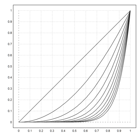
Using an expression does also work. If n is a column vector, Euler will plot all functions.
>plot2d("x^n",a=0,b=1);
Euler has comparison operators, like "==", which checks for equality.
We get a vector of 0 and 1, where 1 stands for true.
>t=(1:10)^2; t==25
[0, 0, 0, 0, 1, 0, 0, 0, 0, 0]
From such a vector, "nonzeros" selects the non-zero elements.
In this case, we get the indices of all elements greater than 50.
>nonzeros(t>50)
[8, 9, 10]
Of course, we can use this vector of indices to get the corresponding values in t.
>t[nonzeros(t>50)]
[64, 81, 100]
There is also a prefix form for nonzeros().
>t[trues t>10]
[16, 25, 36, 49, 64, 81, 100]
As an example, let us find all squares of the numbers 1 to 1000, which are 5 modulo 11 and 3 modulo 13.
>t=1:1000; trues mod(t^2,11)==5 && mod(t^2,13)==3
[4,  48,  95,  139,  147,  191,  238,  282,  290,  334,  381,  425,
433,  477,  524,  568,  576,  620,  667,  711,  719,  763,  810,  854,
862,  906,  953,  997]
EMT is not completely effective for integer computations. It uses double precision floating point internally. However, it is often very useful.
We can check for primality. Let us find out, how many squares plus 1 are primes.
>t=1:1000; length(nonzeros(isprime(t^2+1)))
112
The function nonzeros() works only for vectors. For matrices, there is mnonzeros().
>seed(2); A=random(3,4)
 0.765761  0.401188  0.406347  0.267829
  0.13673  0.390567  0.495975  0.952814
 0.548138  0.006085  0.444255  0.539246
It returns the indices of the elements, which are not zeros.
>k=mnonzeros(A<0.4)
        1         4
        2         1
        2         2
        3         2
These indices can be used to set the elements to some value.
>mset(A,k,0)
 0.765761  0.401188  0.406347         0
        0         0  0.495975  0.952814
 0.548138         0  0.444255  0.539246
The function mset() can also set the elements at the indices to the entries of some other matrix.
>mset(A,k,-random(size(A)))
 0.765761  0.401188  0.406347 -0.126917
-0.122404 -0.691673  0.495975  0.952814
 0.548138 -0.483902  0.444255  0.539246
And it is possible to get the elements in a vector.
>mget(A,k)
[0.267829, 0.13673, 0.390567, 0.006085]
Another useful function is extrema, which returns the minimal and maximal values in each row of the matrix and their positions.
>ex=extrema(A)
 0.267829         4  0.765761         1
  0.13673         1  0.952814         4
 0.006085         2  0.548138         1
We can use this to extract the maximal values in each row.
>ex[,3]'
[0.765761, 0.952814, 0.548138]
This, of course, is the same as the function max().
>max(A)'
[0.765761, 0.952814, 0.548138]
But with mget(), we can extract the indices and use this information to extract the elements at the same positions from another matrix.
>j=(1:rows(A))'|ex[,4], mget(-A,j)
        1         1
        2         4
        3         1
[-0.765761,  -0.952814,  -0.548138]
Almost all functions in Euler work for matrix and vector input too, whenever this makes sense.
E.g., the sqrt() function computes the square root of all elements of the vector or matrix.
>sqrt(1:3)
[1, 1.41421, 1.73205]
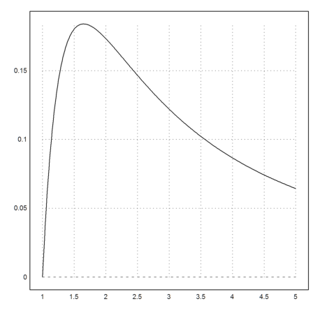
So you can easily create a table of values. This is one way to plot a function (the alternative uses an expression).
>x=1:0.01:5; y=log(x)/x^2; plot2d(x,y):
For the following, we assume, that your already are acquainted with the programming language of EMT.
Functions will only work for vectors, if they return the result using a simple expression, which works for matrices.
>function f(x) := x^3-x; ...
 f(0:0.1:1)
[0,  -0.099,  -0.192,  -0.273,  -0.336,  -0.375,  -0.384,  -0.357,
-0.288,  -0.171,  0]
But if conditional statements or other more complicated statements are involved, the function will no longer work for vectors. It must be vectorized. The easiest way is to use the keyword "map" in the function definition.
Let us define
![]()
>function map f(x) ...
   if x>0 then return x^3
   else return x^2
   endif;
 endfunction
>f(-1:0.5:1)
[1, 0.25, 0, 0.125, 1]
The following method works with all functions.
>fmap(-1:0.5:1)
[1, 0.25, 0, 0.125, 1]
To make sure, your functions are not abused, EMT supports parameter checks. The proper check to prevent vectors is "scalar". Since we use inequalities, we also want the argument to be real.
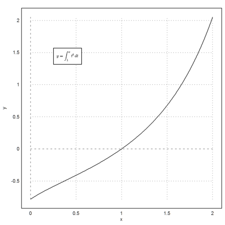
For an example, we compute
![]()
numerically.
>function f(b:real scalar) := integrate("x^x",1,b)
>f(2)
2.05045
To run this function for a vector of values b, it must be vectorize with "map". Or we can map it at run time.
>fmap(2:3)
[2.05045, 13.7251]
The plot functions, as well as some other functions vectorize by default, since they use an adaptive evaluation of the function. So the following works.
>plot2d("f(x)",0,2,xl="x",yl="y");  ...
 textbox(latex("y=\int_1^x t^t \,dt"),x=0.3,y=0.2):
Remember that sqrt is not a matrix function. it simply maps to all elements of the matrix.
>sqrt(B)
        1   1.41421
  1.73205         2
To apply a function to a matrix, we need to compute its eigenvalue decomposition. The function matrixfunction() does this. The matrix gets complex along the way.
>C=matrixfunction("sqrt",B)
 0.553689+0.464394i  0.806961-0.212426i
   1.21044-0.31864i   1.76413+0.145754i
Check it.
>real(C.C)
        1         2
        3         4
The function sort() sorts a row vector.
>sort([5,6,4,8,1,9])
[1, 4, 5, 6, 8, 9]
It is often necessary to know the indices of the sorted vector in the original vector. This can be used to reorder another vector in the same way.
Let us shuffle a vector.
>v=shuffle(1:10)
[7, 8, 3, 2, 9, 6, 4, 5, 10, 1]
The indices contain the proper order of v.
>{vs,ind}=sort(v); v[ind]
[1, 2, 3, 4, 5, 6, 7, 8, 9, 10]
This works for string vectors too.
>s=["a","d","e","a","aa","e"]
a
d
e
a
aa
e
>{ss,ind}=sort(s); ss
a
a
aa
d
e
e
As you see, the position of double entries is somewhat random.
>ind
[4, 1, 5, 2, 6, 3]
The function unique returns a sorted list of unique elements of a vector.
>intrandom(1,10,10), unique(%)
[7,  7,  8,  7,  9,  10,  6,  2,  7,  8]
[2,  6,  7,  8,  9,  10]
This works for string vectors too.
>unique(s)
a
aa
d
e
A simple count of elements with a property can be done with a condition and sum. We have demonstrated that already with primes.
Here is an example with random values. We generate one million random values and count how many of them are positive.
>n=1000000; sum(normal(1,n)>0)/n
0.500167
One could use this method in a loop to get frequencies in intervals. But the function getfrequencies() was made for this. It counts the number of elements of a vector between given bounds.
As an example, we count the number of elements between 0 and 1.
>getfrequencies(normal(1,n),[0,1])/n
0.340712
Here is an example with more than one interval.
>getfrequencies(normal(1,n),-5:5)/n
[4e-005,  0.001412,  0.021666,  0.135988,  0.341105,  0.341552,
0.135571,  0.021352,  0.001285,  2.9e-005]
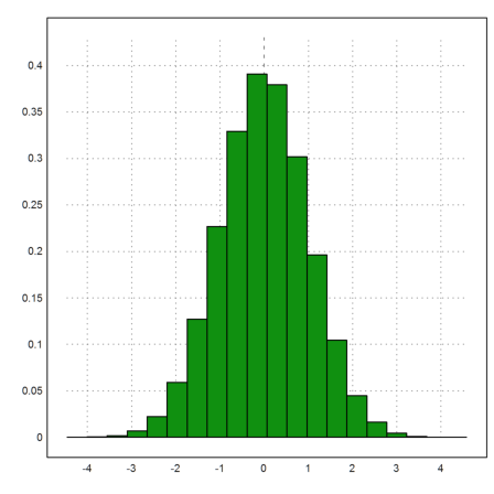
The plot2d uses this method via the histo() function, if the >distribution flag is set.
>plot2d(normal(1,n),>distribution):
The function histo() has simplified arguments to count between the maximal and minimal value of the sample.
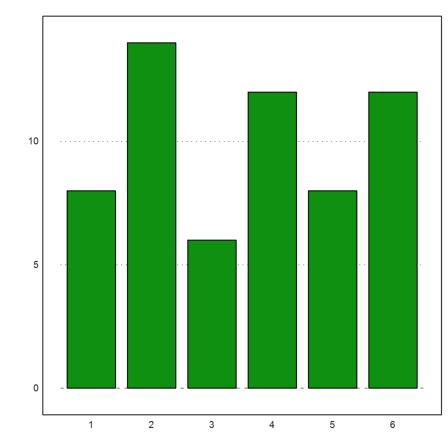
>{x,y}=histo(intrandom(1,60,6),>integer); y,
[8, 14, 6, 12, 8, 12]
>columnsplot(y,lab=1:6):
These functions rely on built-in functions with good efficiency.
One example is the function find(v,x), which finds the elements of x in the intervals given by the sorted vector v with the integer bisection method.
>find(1:5,[0.5,1,3.5,4.5,5,5.5])
[0, 1, 3, 4, 5, 5]
Note that this function returns 0 and n for excessive elements.
For integer values, you can find the indices of x in the sorted vector v with indexofsorted(v,x).
>indexofsorted(1:6,[0,4,1,3,7])
[0, 4, 1, 3, 0]
It returns 0, if the value is not found.
For more elementary functions, have a look into the reference.