Euler has various methods to solve linear and nonlinear optimization problems. Moreover, the methods of Maxima can also be used.
Simplex Algorithm
LPSOLVE package
For a first example, we solve the following problem with the simplex algorithm.
Maximize
![]()
with
![]()
First we define the necessary matrices and vectors.
>shortformat; A:=[1,1,1;2,0,1]
        1         1         1
        2         0         1
>b:=[1;1]
        1
        1
>c:=[2,1,1]
[2, 1, 1]
Now we have to maximize c.x under the condition A.x<=b.
>x:=simplex(A,b,c,>max)
      0.5
      0.5
        0
We can now compute the maximal value.
>c.x
1.5
If <check is off, the Simplex function returns the solution and a flag. If the flag is 0, the algorithm found a solution. If >check is on (the default), the function throws an error, if the problem is not bounded or not feasible.
>{x,r}:=simplex(A,b,c,>max); r,
0
For Maxima, we have to load the simplex package first.
>&load(simplex);
Then we can solve the problem in symbolic form.
>&maximize_lp(2*x+y+z,[x>=0,y>=0,z>=0,x+y+z<=1,2*x+z<=1])
                       3              1      1
                      [-, [z = 0, y = -, x = -]]
                       2              2      2
An integer solution can be computed with the branch and bound algorithm using the function "intsimplex".
>x:=intsimplex(A,b,c,>max,>check)
        0
        1
        0
>c.x
1
The function ilpsolve from the LPSOLVE package (see below for details and more examples) gets the same solution.
>ilpsolve(A,b,c,>max)
        0
        1
        0
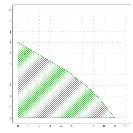
In the case of two variables, the function feasibleArea can compute the corners of the feasible points, which we can then plot.
>A:=[1/10,1/8;1/9,1/11;1/12,1/7]; b:=[1;1;1]; xa:=feasibleArea(A,b); ...
 plot2d(xa[1],xa[2],filled=1,style="/",a=0,b=10,c=0,d=10);  ...
   insimg();
>x=simplex(A,b,[5,8],max=1); fracprint(x);
    60/13
    56/13
>plot2d(x[1],x[2],add=1,points=1):

Here is an integer solution.
>intsimplex(A,b,[5,8],max=1)
        5
        4
>plot2d(5,4,points=true,style="ow",add=true):

For a demonstration, we solve this system using the pivotize function of Euler, which does one step of the Gauß or the Gauß-Jordan algorithm. We use the Gauß-Jordan form, since it is well suited for this problem.
The problem in the form
![]()
is written in the following scheme.
>shortestformat; A := [1,1,1;4,0,1]; b := [1;1]; M := (A|b)_(-[2,1,1])
     1      1      1      1
     4      0      1      1
    -2     -1     -1      0
For the output of the Gauß-Jordan scheme, we need the names of the variables, and for book keeping we need an index vector 1:6 for the current permutation of the variables.
>v := ["s1","s2","","x","y","z"]; n := 1:6;
With that information, we can print the scheme.
>gjprint(M,n,v)
                   x         y         z
        s1     1.000     1.000     1.000     1.000
        s2     4.000     0.000     1.000     1.000
              -2.000    -1.000    -1.000     0.000
The Simplex algorithm now requires to exchange x for s2. If we add the variable names, the scheme is automatically printed after each step.
Note that the algorithm changes M and n. So, be careful not to run this command twice!
>gjstep(M,2,1,n,v);
                  s2         y         z
        s1    -0.250     1.000     0.750     0.750
         x     0.250     0.000     0.250     0.250
               0.500    -1.000    -0.500     0.500
Next, we have to exchange y for s2.
>gjstep(M,1,2,n,v);
                  s2        s1         z
         y    -0.250     1.000     0.750     0.750
         x     0.250     0.000     0.250     0.250
               0.250     1.000     0.250     1.250
This finishes the algorithm, and we find the optimal values
![]()
We can extract the solution with gjsolution().
>fracprint(gjsolution(M,n))
[1/4, 3/4, 0]
Euler has some methods for non-linear optimization.
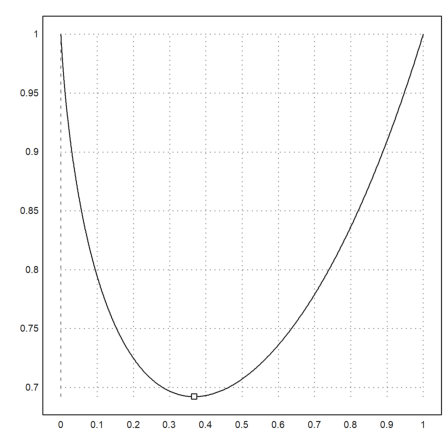
For one dimensional minimization or maximization of a function, there are fmin and fmax. These functions use a clever trisection, and work for convex (resp. concave) functions.
>longformat; xm := fmin("x^x",0,1)
0.367879431153
>plot2d("x^x",0,1); plot2d(xm,xm^xm,>points,>add):
We can also solve with Maxima for the zero of the derivative.
>&assume(x>0); &solve(diff(x^x,x)=0,x)
                                - 1   x
                          [x = E   , x  = 0]
So the point is actually exp(-1).
>exp(-1)
0.367879441171
Of course, we can use any zero finding method of Euler, computing the derivative in Maxima.
>secant(&diff(x^x,x),0.1,1)
0.367879441171
A numerical solution would imply the numerical computation of the derivative. So we program that for any expression or function expr.
>function g(x,expr) ...
 return diff(expr,x)
 endfunction
Then we call the secant method, passing the expression as an extra argument to g.
>secant("g",0.1,1;"x^x")
0.367879441172
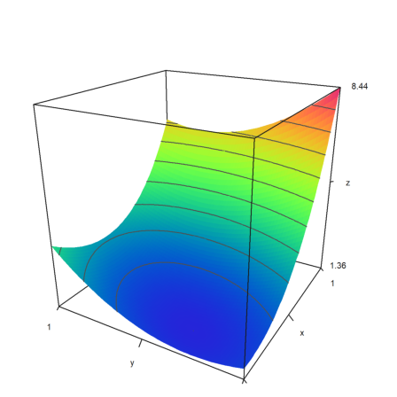
Next, we try a multidimensional minimization. The function is
![]()
>expr:="y^2-y*x+x^2+2*exp(x)";
If we plot it in 3D we can vaguely see the minimum.
>plot3d(expr,>levels,angle=-60°,>spectral):
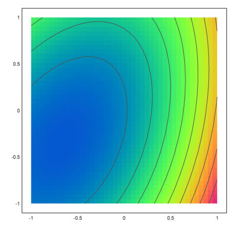
It is better to use a contour plot. The minimum is clearly visible.
>plot2d(expr,>levels,grid=4,>hue,>spectral):
Now we try to solve the problem symbolically.
>expr &= y^2-y*x+x^2+2*exp(x)
                          2            x    2
                         y  - x y + 2 E  + x
However, Maxima fails here. The system is too complex.
>&solve(gradient(expr,[x,y]))
Maxima said:
algsys: tried and failed to reduce system to a polynomial in one variable; give up.
 -- an error. To debug this try: debugmode(true);

Error in:
&solve(gradient(expr,[x,y])) ...
                            ^
The Nelder-Mead method solves this very well. We need to write a function, evaluation the expression at a 1x2 vector.
>function f([x,y]) &= expr
                          2            x    2
                         y  - x y + 2 E  + x
Now we can call Nelder-Mead, passing the expression to the function.
>res:=nelder("f",[0,0])
[-0.677309026763, -0.338655071019]
Another method without derivatives is the Powell minimization. It is a very good method.
>powellmin("f",[0,0])
[-0.677309310645, -0.338654643461]
If we have the gradient and the Hesse matrix of f, we can solve for the gradient.
There is a wrapper function for the Newton method in two variables, which needs expressions for both components of the function. We use it to find the critical point of our function.
>mxmnewtonfxy(&diff(expr,x),&diff(expr,y),[1,0])
[-0.677309305781, -0.338654652891]
If we have the derivatives, we can start the Newton method or get a guaranteed inclusion for the solution.
First, we define a function, evaluating the derivative (gradient) of f.
>function Jf ([x,y]) &= gradient(f(x,y),[x,y])
                               x
                     [- y + 2 E  + 2 x, 2 y - x]
Let us check our solution.
>Jf(res)
[1.25963816155e-06, -1.11527498425e-06]
Then we define the derivative of Jf which is the Hesse matrix of f.
>function Hf ([x,y]) &= hessian(f(x,y),[x,y])
                          [    x          ]
                          [ 2 E  + 2  - 1 ]
                          [               ]
                          [   - 1      2  ]
Compute the Hesse matrix at the solution.
>Hf(res)
      3.01596424214                  -1
                 -1                   2
Now, check if it is positive definite. This is already a proof for a local minimum.
>re(eigenvalues(Hf(res)))
[3.62960854521, 1.38635569693]
The Newton algorithm finds the minimum easily.
>newton2("Jf","Hf",[0,0])
[-0.677309305781, -0.338654652891]
As an alternative, the Broyden algorithm needs only a function, in our case the gradient function.
>broyden("Jf",[0,0])
[-0.677309305781, -0.338654652891]
We can now use the interval Newton method in several dimensions to obtain a guaranteed inclusion of the critical point.
>ires:=inewton2("Jf","Hf",[0,0])
[ ~-0.6773093057811569,-0.6773093057811558~,
~-0.3386546528905785,-0.33865465289057783~ ]
This is a method for non-linear or linear minimization of a a convex function with linear restrictions.
Let us try a random linear example first with 1000 conditions and two variables.
>A=1+random(1000,2); b=150+random(1000,1)*100;
>A=A_-id(2); b=b_zeros(2,1);
>c=[-1,-1];
The Simplex algorithm gets the following result.
>longest simplex(A,b,c,eq=-1,<restrict,>min,>check)'
67.26867866525664 13.52921155992493
For the Newton-Barrier method, we need the gradient and the Hessian of f.
>function f([x,y]) &= -x-y;
>function df([x,y]) &= gradient(f(x,y),[x,y]);
>function Hf([x,y]) &= hessian(f(x,y),[x,y]);
New we can start the Newton-Barrier method.
>longest newtonbarrier("f","df","Hf",A,b,[1,1])
67.26867866501856 13.52921156015715
Let us try a nonlinear target function. We maximize
![]()
Since we need a convex function, we take
![]()
instead, and minimize this function.
>function f([x,y]) &= 1/(x*y);
>function df([x,y]) &= gradient(f(x,y),[x,y]);
>function Hf([x,y]) &= hessian(f(x,y),[x,y]);
>longest newtonbarrier("f","df","Hf",A,b,[1,1])
41.202676464346 39.25233817005504
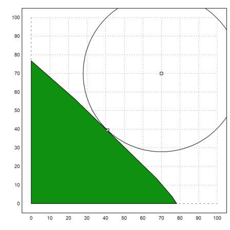
For another example, we search the point of minimal distance to (70,70).
>X=feasibleArea(A,b);  ...
 plot2d(X[1],X[2],a=0,b=100,c=0,d=100,>filled); ...
 x0 &:= 70; y0 &:= 70; plot2d(x0,y0,>points,>add):

>function f([x,y]) &= (x-x0)^2+(y-y0)^2
                                2           2
                        (y - 70)  + (x - 70)
>function df([x,y]) &= gradient(f(x,y),[x,y])
[2 (x - 70), 2 (y - 70)]
>function Hf([x,y]) &= hessian(f(x,y),[x,y])
                               [ 2  0 ]
                               [      ]
                               [ 0  2 ]
We can now start the Newton-Barrier method.
>X=newtonbarrier("f","df","Hf",A,b,[1,1]);
Let us plot the result.
>x1=X[1]; y1=X[2]; plot2d(x1,y1,>points,>add); ...
 r=sqrt((x1-x0)^2+(y1-y0)^2); ...
 plot2d(x0,y0,>points,>add); ...
 t=linspace(0,2pi,500); plot2d(x0+r*cos(t),y0+r*sin(t),>add):
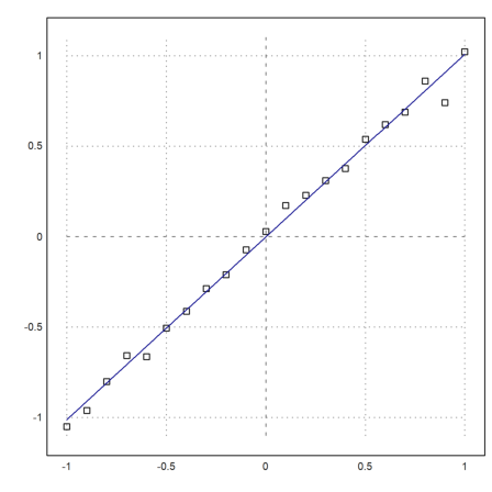
Next, we want to demonstrate a linear fit.
First we assume that we have measurements of y=x with a normally distributed error.
>x:=-1:0.1:1; y:=x+0.05*normal(size(x));
>plot2d(x,y,style="[]",a=-1,b=1,c=-1.1,d=1.1,points=1);
Now we fit a polynomial of degree 1 to this.
>p:=polyfit(x,y,1), plot2d("evalpoly(x,p)",add=1,color=4):
[-0.00201947657644, 1.0098236374]
We compute the sum of the squares of the errors, and the maximum error.
>sum((evalpoly(x,p)-y)^2), max(abs(evalpoly(x,p)-y))
0.0519010499483
0.166766952777
Assume, we want to minimize the maximum error. We use Nelder-Mead again.
>function f(p,x,y) := max(abs(evalpoly(x,p)-y))
>q:=neldermin("f",[0,0];x,y)
[-0.0034048233685, 0.945518925639]
Let us compare. This time, the first error must be larger, and the second smaller.
>sum((evalpoly(x,q)-y)^2), max(abs(evalpoly(x,q)-y))
0.0837815916995
0.1075073654
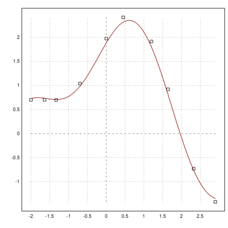
For non-linear fits, there is the function modelfit(), which uses the Powell method by default.
You need to provide a model function model(x,p). This function must vectorize (map) to x and p.
>function model(x,p) := p[1]*cos(p[2]*x)+p[2]*sin(p[1]*x);
We provide some data.
>xdata = [-2,-1.64,-1.33,-0.7,0,0.45,1.2,1.64,2.32,2.9]; ...
 ydata = [0.699369,0.700462,0.695354,1.03905,1.97389,2.41143, ...
   1.91091,0.919576,-0.730975,-1.42001];
Now all we need to do is to call modelfit() with an initial guess. We can use the stable Nelder-Mead algorithm or Powell's minimization.
>pbest=modelfit("model",[1,0.2],xdata,ydata,>powell)
[1.88185085219, 0.700229817942]
>plot2d(xdata,ydata,>points); plot2d("model(x,pbest)",color=red,>add):
The function modelfit() uses the L2-norm by default. But we can just as well use any other norm.
>modelfit("model",[1,0.2],xdata,ydata,p=0)
[0.41027821664, 0.783198346252]
This function can also be used for multi-variate fits. We take a linear model.
>function model(X,p) := p.X;
Here x is a matrix of data points, one in each column, and p is a parameter vector.
We now generate such a vector and noisy data, and use fit() to find the best fit. Without the noise, the correct result is [1,1].
>X=random(10,2); b=sum(X)+0.1*normal(10,1); fit(X,b)
      1.00378096271
     0.956035889705
We can get the same result with modelfit().
>modelfit("model",[1,1],X',b')
[1.00378124605, 0.95603561523]
But we can also get the best fit in the sup-norm with p=0.
>modelfit("model",[1,1],X',b',p=0)
[0.93032137681, 1.02153647642]
The following example is from the Rosetta page. You have the following items.
>items=["map","compass","water","sandwich","glucose", ...
   "tin","banana","apple","cheese","beer","suntan creame", ...
   "camera","t-shirt","trousers","umbrella","waterproof trousers", ...
   "waterproof overclothes","note-case","sunglasses", ...
   "towel","socks","book"];
These items have the following weights each.
>ws = [9,13,153,50,15,68,27,39,23,52,11, ...
   32,24,48,73,42,43,22,7,18,4,30];
And for your trip, they have the following values.
>vs = [150,35,200,160,60,45,60,40,30,10,70, ...
   30,15,10,40,70,75,80,20,12,50,10];
You are not allowed to take more weight than a total of 400 with you, and you can only take one item of each kind.
The model is
![]()
![]()
This can immediately be translated into an integer linear program.
>A=ws_id(cols(ws)); b=[400]_ones(cols(vs),1); c=vs;
The matrix A contains the restriction in the first row, followed by rows of the type
![]()
>sol = intsimplex(A,b,c,eq=-1,>max,>check);
The solution is to take the following items.
>items[nonzeros(sol)]
map
compass
water
sandwich
glucose
banana
suntan creame
waterproof trousers
waterproof overclothes
note-case
sunglasses
socks
Euler does also contain the LPSOLVE library, ported to Euler by Peter Notebaert.
The function ilpsolve uses this package. If you need the package in other form, you will have to start it by loading lpsolve.e. See Notebaert's examples in the user directory for more information.
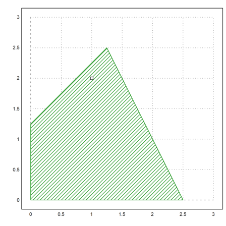
We solve a first problem. The syntax is similar to intsimplex. The restrictions are
![]()
and we maximize
![]()
>longformat;
>f := [-1, 2]; // target function
>A := [2, 1;-4, 4]; // restriction matrix
>b := [5; 5]; // right hand side
>e := -[1; 1]; // type of restrictions (all <=)
Solve with LP solver.
>x := ilpsolve(A,b,f,e,max=1)
                  1
                  2
Compare with the slower intsimplex function.
>intsimplex(A,b,f,e,max=1)
                  1
                  2
Draw the feasible area.
>xa := feasibleArea(A,b); ...
 plot2d(xa[1],xa[2],filled=1,style="/",a=0,b=3,c=0,d=3); ...
 plot2d(x[1],x[2],points=1,add=1); insimg();
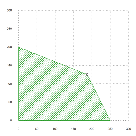
We can use LPSOLVE also for non-integer programming.
>f = [50, 100]; ...
 A = [10, 5; 4, 10; 1, 1.5]; ...
 b = [2500; 2000; 450]; ...
 e = [-1; -1; -1]; ...
 x=ilpsolve(A,b,f,e,i=[],max=1) // i contains the integer variables
              187.5
                125
>xa:=feasibleArea(A,b); ...
 plot2d(xa[1],xa[2],filled=1,style="/",a=0,b=300,c=0,d=300); ...
 plot2d(x[1],x[2],points=1,add=1):
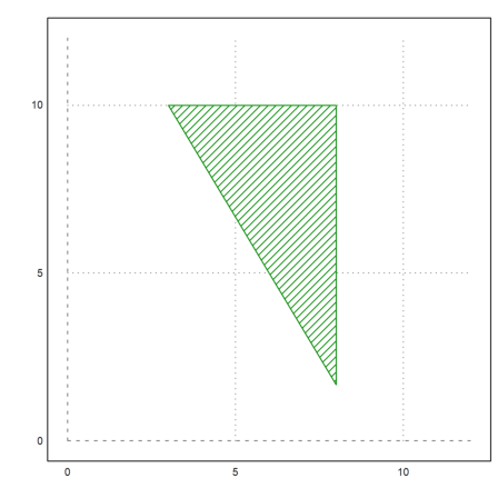
Next, we have a lower bound A.x >= b, and some upper bounds for the variables. Furthermore, we minimize the target function. lpsolve can add such restrictions in a special form.
>f = [40, 36]; ...
 A = [5, 3]; ...
 b = [45]; ...
 e = 1; ...
 {v,x} = ilpsolve(A,b,f,e,vub=[8,10],max=0);
>v
                  8
                  2
>x
392
To solve this in intsimplex, we can add the restrictions to the matrix A.
>intsimplex(A_id(2),b_[8;10],f,e_[-1;-1],max=0)
                  8
                  2
The feasible area looks like this. It is always computed with inequalities of the form A.x <= b. So we must modify our matrix again.
>xa:=feasibleArea((-A)_(id(2)),(-b)_[8;10]); ...
 plot2d(xa[1],xa[2],filled=1,style="/",a=0,b=12,c=0,d=12);  ...
   insimg();
Now, we restrict only one of the variables to integer.
>f = [10, 6, 4]; ...
 A = [1.1, 1, 1; 10, 4, 5; 2, 2, 6]; ...
 b = [100; 600; 300]; ...
 e = [-1; -1; -1]; ...
 ilpsolve(A,b,f,e,i=[2],max=1)
      35.4545454545
                 61
                  0
>intsimplex(A,b,f,e,max=1,i=[2])
      35.4545454545
                 61
                  0
Let us try a huge problem with random restrictions.
>seed(0.2); A=random(100,10); b=random(100,1)*10000; c=ones(1,10);
First the non-restricted solution.
>ilpsolve(A,b,c,>max,i=[])
                  0
                  0
                  0
                  0
      9.46772793089
                  0
      208.267610249
                  0
                  0
      21.4674357674
Then the integer solution.
>ilpsolve(A,b,c,>max)
                  0
                  0
                  4
                  0
                  8
                  0
                204
                  0
                  0
                 23