There have been a lot of small fixes in the documentation and a change in the Visual C++ version which are not documented here.
The file hosting has also been changed. Details are on the home page of EMT.
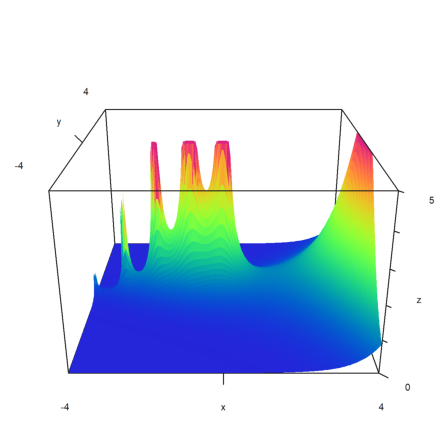
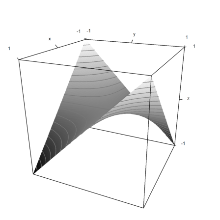
Fixed a small error in the Gamma function.
>x=-4:0.05:4; y=x';
>h=min(abs(gamma(x+I*y)),5);
>plot3d(x,y,h,>spectral,angle=0°,zoom=3):
There is now a prefix version of nonzeros() named "sel" (for "select").
>a=random(10)
[0.52143,  0.428893,  0.168134,  0.182742,  0.288048,  0.750042,
0.472935,  0.324407,  0.340388,  0.195494]
>sel a>0.5
[1, 6]
>a[sel a>0.5]
[0.52143, 0.750042]
All key combinations Ctrl-Alt have been changed to Ctrl-Shift. This seems to be less confusing for the user.
I worked on the example about the DOF of an ideal lens, making it much clearer and adding a formula for the Bokeh.
>load dof
Functions for DOF, hyperfocal distance and Bokeh.

startDOF, endDOF: computes depth of field (DOF)
DOF: prints ranges of DOF
hyperfocal: computes hyperfocal distance
bokeh: computes quality of Bokeh (blurriness at infinity)

lens: prints various parameters for a specific lens

For another calculator:

  https://www.photopills.com/calculators/dof
>lens(2m,85mm,2.8)
35mm equival focal length      : 85.0 mm
35mm equival F-stop            : F 2.8
Focussed distance              : 2.0 m

Start of DOF                   : 1.96 m
End of DOF                     : 2.05 m
Total DOF                      : 0.09 m

Hyperfocal distance            : 86.1 m
Sharpness from                 : 43.0 m

Bokeh quality                  : 6.0%
The download is now possible only via Sourceforge. This is slower, but the users have more trust and it is easier to maintain.
I also tried to host the web page on Sourceforge. Unfortunately, uploading or updating new content is very slow. Moreover, there is a problem with the time stamps, so that all files are refreshed at each update. Additionally, the web pages on Sourceforge are not SSL encoded. For the time being, the web page of Euler Math Toolbox will be hosted on Strato.
Some work in the documentation, including a better outline of the parameters for plot2d and plot3d.
Fixed the weekday function for sundays.
>weekday(day(2021,12,12),>name)
Sunday
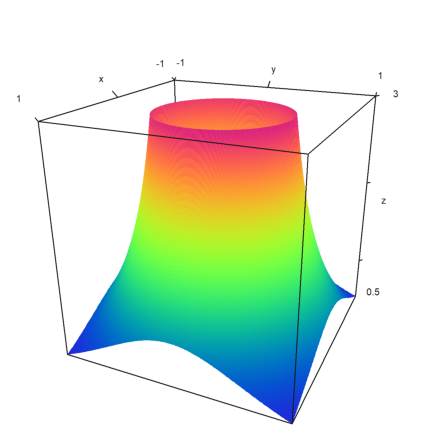
Fixed the "limits" parameter of plot3d for scaled output, and added more documentation for this parameter. "limits" should be 1x2 vector [zmin,zmax], and will cut off exceeding z-values. It works only for functions with hue.
>plot3d("min(1/(x^2+y^2),3)",>zhue,>spectral,n=200,limits=[0,2.95]):
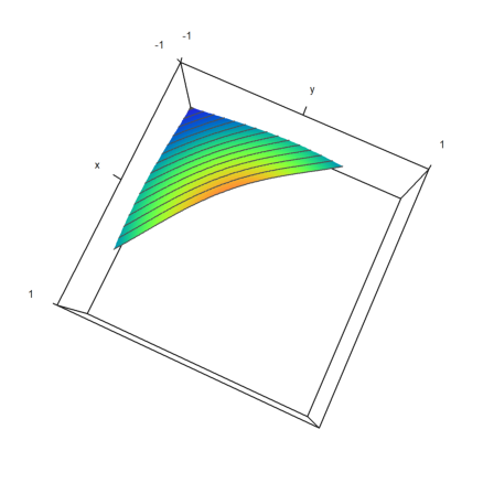
Now, limits should also work if the level values are computed in any other way.
>x=linspace(-1,1,100); y=x'; z=exp(-x^2-y^2); ...
 plot3d(x,y,z,>zhue,>spectral,values=x+y, ...
   levels=-2:0.1:0,limits=[-2,0],height=80°):
There is now a function weekday(). It can compute the weekday (1=Monday, 7=Sunday), or its name in English.
>printnow()
Sonntag, 12. Dezember 2021 16:43:44
>weekday(daynow()), weekday(daynow(),>name)
0
Sunday
>weekday(day(2022,1,1),>name)
Saturday
In Windows 11, the UTF conversion started to produce problems. The reason is the system wide support for UTF-8. This is currently in Beta and I suggest switching it off for Euler Math Toolbox. It is in the administrative settings for time and language.
If you do want to use the UTF-8 settings, you can set your codepage in the settings now. It is used to translate from an to UTF-8. The European codepage is 1250. If you set 0 here, the system default will be used.
I had to change some shortcuts.
EMT can now produce Markdown output to "*.md" files. The output is similar to the HTML export, but the output is easier to read and modify.
You can open Markdown files with various editors, free and payware. Moreover, there are plugins in Chrome and Edge if you allow accessing URLs. It is possible to compile the files to HTML with command line tools. Note, that Latex formulas are exported directly, and ususally interpreted using MathJax in the Markdown display.
Currently, it is not possible to use Markdown language in comments. The reason for this is that EMT is line oriented and cannot change fonts within a line. So, it does not make sense to implement the Markdown language fully. The comment syntax is not difficult to learn anyway.
A lot of work and changes in the documentation.
Again a lot of work on the tutorials, the examples, and the help texts.
Some improvements have been done to the help function, including some changes in the help menu. The man help now contains an overview and a help on the user interface.
I also improved the tutorial about Tiny C programming and a lot of other tutorials.
The file "util/EMT.xml" contains now a syntax import for Notepad++.
EMT can now handle Python 3. I could test it with Python 3.8. I suggest installing a version from the main Python site.
https://www.python.org/downloads/release/python-380/
It might be necessary to add the directory of Python to the path. At least, EMT needs to be able to use python38.dll.
To enable Python38, uncheck "Use Python 2.7" in the program options before using Python.
Fixed the function drop(v,i) which now works only for row vectors v and i. The index vector can contain negative indices. Note that the index vector will be sorted by this function.
>v=[10:20]
[10, 11, 12, 13, 14, 15, 16, 17, 18, 19, 20]
Drop the last element and the element at positions 2 and 3.
>drop(v,[-1,2,3])
[10, 13, 14, 15, 16, 17, 18, 19]
For matrices, use droprows() or dropcols(),
>droprows([1,2,3;4,5,6],1)
[4, 5, 6]
>dropcols([1,2,3;4,5,6],2)
            1             3
            4             6
There are the new functions butlast() and butfirst() now.
>butlast(1:10), butfirst(1:10)
[1,  2,  3,  4,  5,  6,  7,  8,  9]
[2,  3,  4,  5,  6,  7,  8,  9,  10]
Alt-Backspace now deletes the commands as before and adds it to the undo buffer. But the undo buffer is cleared now for each delete unless the key is pressed several times without changing the current line. This allows deleting and inserting several successive lines.
Alt-U inserts the current undo at the current position in the notebook (i.e., in front of the current line). It also clears the undo buffer.
For more control, use Cut and Paste.
Internal update of the web page.
Extended "map" so that the result of the function does not have to be either real or complex. In previous versions, "map" took the first function result to determine the type of the resulting vector. If any successive result was different the result was an error.
>function map f(x) ...
 if x~=0 then return 0; // real result
 else return 2*x; // might be complex
 endif
 endfunction
This works, even if the first vector element of the result is real.
>f((0:2)*I)
[ 0+0i , 0+2i, 0+4i ]
Or if there is a real result between the complex results.
>f((-1:1)*I)
[ 0-2i, 0+0i , 0+2i ]
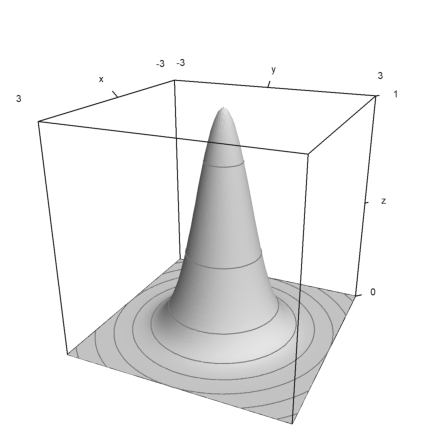
The parameter >hue for plot3d is no longer automatically changed to >zhue if the plot contains z-levels. This looks better for plots which would otherwise be very dark in larger areas.
>plot3d("exp(-x^2-y^2)",r=3,levels=exp(-(0:0.5:5)^2),>hue,n=100):
The default >zhue is not computed by the light shining on the plot, but by the z-values.
>plot3d("x*y",levels=-2:0.1:2):
Fixed a crash when nelder() was called without arguments. Thanks to Th. Risse.
>errorlevel("nelder")
26
Improved the documentation of the elliptical functions.
>help ellrf
ellrf is an Euler function.

function map ellrf (x, y, z, eps)

Default for eps : none

Function in file : C:\euler\util\functions

Carlson's elliptic integral of the first kind RF (x; y; z).

The iteration is implemented in the Euler language.

x, y, and z must be non-negative, and at most one can be zero.
Computes

 1/2 integrate(1/sqrt((t+x)*(t+y)*(t+z)),t=0..inf)

See: ellrd, ellf
Fixed 13 and 10 in strings. Both generate a new line in the output now, as well any sequence 13/10 or 10/13.
>"A"+char(10)+"B"+char(13)+"C"+ ...
   char(10)+char(13)+"D"+char(13)+char(10)+"E"
A
B
C
D
E
This is just a cleanup of the code.
Fixed F11 (to resize the windows to full screen automatically) for getting the cursor position and screen length correctly.
Euler has now been compiled with "Visual Studio Cummunity 2019". The source file contains the project file "euler.vcxproj".
The formats "shortformat", "short" and "shortest" have been updated.
>A=normal(5,5); short A,
 -0.42429   0.65886  0.090315   0.48911    1.3535
  0.96684   0.43548   -1.1129    1.2365   0.78854
  0.77879  0.035098   -0.1664 -0.053575  -0.33024
  -0.5082   0.15857   -1.6755  -0.62694   0.11508
  0.58619   0.88865    1.4146   0.66452   -2.0918
The download is no longer from my site, but from the Files section at SourceForge. The reason for this change is that the files are checked thouroughly by SourceForge for viruses. It becomes important more and more to prove that the download is clean.
The fonts are now saved again.
The official forum for Euler Math Toolbox is now at SourceForge at
https://sourceforge.net/p/eumat/discussion/
I will also try to keep the files section in SourceForge up to date with the most recent version. The HTML files remain on my server at Strato, as well as the downloads.
The 32-bit version will no longer be updated, or only at very special request. The version of May 2017 will remain on the server.
Moreover, there will no longer be a Maxima-less version of Euler Math Toolbox. The internet is fast enough now for a download of the full version (around 100 MB).
Now the right mouse button works in the following ways:
(1) Clicking into a comment opens the comment window.
(2) Clicking into a program opens the internal editor.
Euler does no longer use the registry. Instead, the configuration is written to the file ".euler.cfg" in the home directory of the user. For old users, the registry is read once to keep old settings.
Fixed the drop routine. It does no longer sort the vector of elements to be dropped.
>a=1:10; b=[6,5,4]; drop(a,b)
[1, 2, 3, 7, 8, 9, 10]
>b
[4, 5, 6]
Fixed frac(x) which now works for very small elements, just like fraction and fracprint().
>frac(1e-15)
0
Added an Euler file for the simplex algorithm in Gauss-Jordan form. See the documentation.
>// load pivp
The help window now searches for strings automatically if no topic is found.
The function mset() is now fixed and works, even if there is nothing to set.
>v=dup(1:3,2); mset(v,mnonzeros(v<0),0)
            1             2             3
            1             2             3
There is no v[i]<0. But in the following v, there are v[i]<0.
>v=dup(-1:1,2); mset(v,mnonzeros(v<0),0)
            0             0             1
            0             0             1
Note how mnonzeros(v<0) works. It returns the indices, where this is true.
>mnonzeros(v<0)
            1             1
            2             1
For vectors, you can also use the following.
>v=-5:5; v[nonzeros(v<0)]=0
[0, 0, 0, 0, 0, 0, 1, 2, 3, 4, 5]
There is a new modifier "usenan". It evaluates the command with "errors off" and sets "errors on" afterwards.
>usenan log(-3:3)
[NAN, NAN, NAN, NAN, 0, 0.693147, 1.09861]
E.g., let us compute sum(1/v), where v is not 0.
>v=0:5; usenan w=1/v
[NAN, 1, 0.5, 0.333333, 0.25, 0.2]
Now, we eliminate the NANs before we sum up.
>sum(w[nonzeros(!isNAN(w))])
2.28333333333
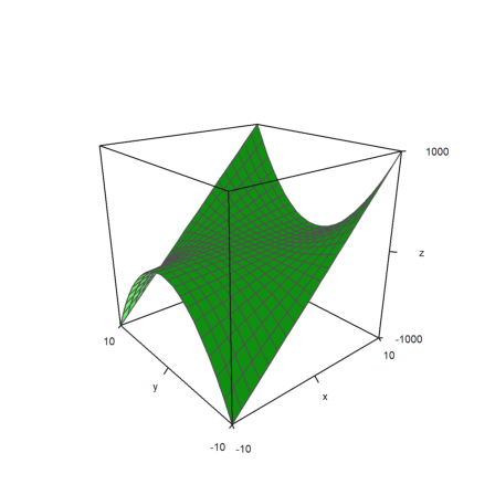
The plot3d(x,y,z) routine for plotting surfaces now respects >zscale. In this case, z is assumed to be a function value. The function is scaled so that everything fits into a unit cube. But the function values are scaled with respect to x and y first.
>x=-10:10; y=x'; z=x*y^2; plot3d(x,y,z,>zscale,angle=-40°,zoom=2):
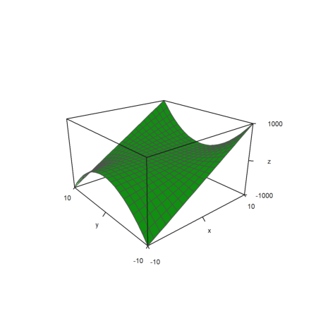
The value of zscale is used to scale into that direction.
>plot3d(x,y,z,zscale=0.6,angle=-40°,zoom=2):
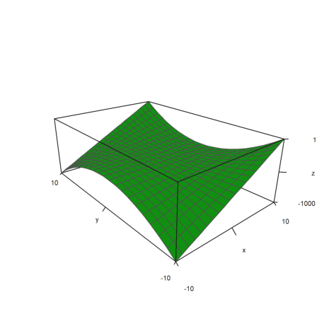
Additionally, scale=[sx,sy,sz] can be used.
>plot3d(x,y,z,>zscale,scale=[1,1.5,0.5],angle=-40°,zoom=2):
I have removed the ancient function scale() and replaced it with something more useful. Now scale(A) scales the matrix A into [epsilon,1].
>sort(scale(random(10)))
[2.85806e-12,  0.114778,  0.157947,  0.236588,  0.452789,  0.560649,
0.61685,  0.767075,  0.992234,  1]
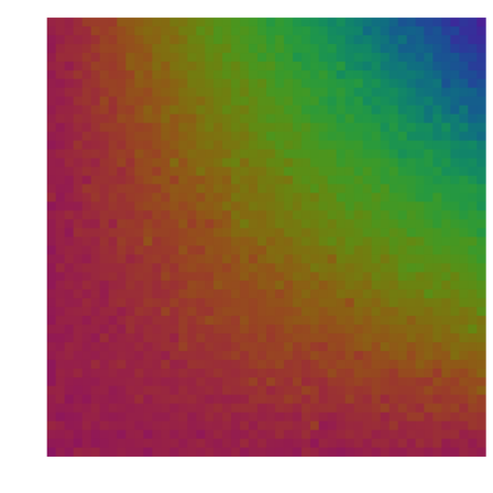
This is useful for plots. E.g., we disturb the matrix (i*j) randomly. To get spectral colors, we scale the result to [0,1]. This will be a noisy plot of x*y.
>n=50; A=(1:n)*(1:n)'; clg; plotrgb(getspectral(scale(A+n*normal(n,n)))):
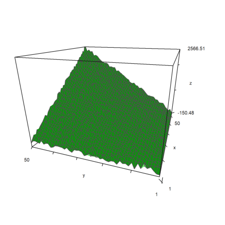
If you plot the same with plot3d, you do not need to scale, because plot3d() has its own scaling parameter. It needs to print the labels correctly.
>plot3d(A+n*normal(n,n), ...
   scale=[80,80,1],angle=-70°,center=[0,0,0.5],zoom=1.7):
I have also expanded the function crossproduct(). It will work now for matrices with three rows, and it will return the results in such a matrix.
>v=[2,3,4]'; crossproduct(v,v|(v+1))
            0            -1
            0             2
            0            -1
I also added the Gram determinant. It computes the volume of the parallelotope spanned by the columns of a matrix. For two vectors in three dimensions, this happens to be the same as the cross product.
>w=[3,4,-2]'; gramdet(v|w), norm(crossproduct(v,w))
27.2213151776
27.2213151776
The generalized cross product is added too. It returns a vector perpendicular to all n-1 columns of a matrix with n rows. The length of the vector is equal to the area of the parallelotope spanned by the columns.
>M=normal(4,3); v=vectorproduct(M); M'.v, norm(v), gramdet(M)
            0
            0
            0
0.522759022566
0.522759022566
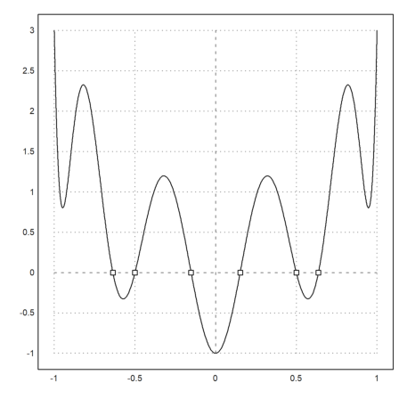
I added a function fzeros() which finds all zeros of another function in an interval. It makes use of fextrema() and bisectin().
>fx := "cheb(x,10)+2*x^2"; ...
 plot2d(fx,-1,1); w=fzeros(fx,-1,1); plot2d(w,fx(w),>points,>add):
Due to user demand, there is now a Python mode.
>pythonmode on
Python mode is on
From now on every command, is interpreted as a Python command.
>print "This is Python"
This is Python
Multi-lines work as expected. For Python control structures, you must use multi-lines and indentation.
>n=1 ...
 for k in range(2,40): ...
   n=n*k ...
 print n
20397882081197443358640281739902897356800000000
You can use "function python" for multi-line commands too.
>function python  ...
 n=1
 for k in range(2,40):
    n=n*k
 print n
 endfunction
20397882081197443358640281739902897356800000000
You can define functions with "def" in a multi-line command, or as a "python" function.
>def fak(n): ...
   m=1 ...
   for k in range(2,n): ...
     m=m*k ...
   return m
>print fak(40)
20397882081197443358640281739902897356800000000
The alternative is a python function. That would work outside of python mode too.
>function python fak(n) ...
 m=1
 for k in range(2,n):
   m=m*k
 return m
 endfunction
>print fak(40)
20397882081197443358640281739902897356800000000
Maxima lines work too.
>:: 40!
815915283247897734345611269596115894272000000000
EMT works in this mode with "euler".
>euler 40!
8.15915283248e+47
>pythonmode off
Python mode is off
Note that the Python function as defined with "function python fak(n)" is available outside of Python mode now.
>fak(40)
2.03978820812e+46
Some Maxima replacements got fixes to make things more logical. To escape any character in a symbolic expression you can now use \c.
The following defines an infix operator | in Maxima which simply multiplies to values. We need to escape the | and the := in symbolic expressions.
>&infix("\|",115); &a\|b \:= a*b; &3\|4
12
It might be easier to use the direct mode for this as written in the Maxima documentation.
>::: infix("|",115)$ a|b := a*b$ 3|4
12
Furthermore, &!... will prevent any replacements in the symbolic expression. (If you need an expression to start with ! enter &!!...)
>&!(a+b)|(a+b)
                                      2
                               (b + a)
There are some changes in the web pages that are installed with EMT. Now, links on these pages show the installed documentation. There is a link to the web site in the link box. The PDF files are also linked to the web site, as well as the search results.
There have been some fixed in the Maxima interface, nothing the ordinary user would notice.
In purely symbolic functions := is now replaced by : to make those mre readable. If you do not want this use the direct mode ":::".
>function cfx(n) &&= block([x], ...
   for i:=1 thru n do x:=1+1/x, x);
>&cfx(3)
                                1
                            --------- + 1
                              1
                            ----- + 1
                            1
                            - + 1
                            x
It is now possible to define purely symbolic strings with the following syntax. Note that s in the following definition is a string, not an expression.
>s &&= ""sin(pi/5)""; &s
sin(pi/5)
The function frac() got a a local epsilon.
>frac(1/7+1e-9,eps=1e-4), frac(1/7+1e-9)
1/7
20408163/142857140
Even more improvements in the documentation and a more concise web page. Nowadays, people do not bother to read long texts on home pages.
The following does work now.
>A=[1,2;0,1]; A.A^2.A
            1             8
            0             1
Previously, A^2.A did not work because "2." was taken as the number "2".
I also fixed the following which was not working. It is an abuse of the matrix product anyway.
>pi.pi
9.86960440109
Note that "2.A" does not work due to incompatible dimensions. You have to write
>2*A
            2             4
            0             2
This is only an update of the documentation with many error fixes and improvements. There is also a new tutorial intended for teachers.
The code for the redraw of the screen has been changed a little bit. This should prevent flicker on weaker machines. I hope it has no serious side effects.
Besides some minor fixes in the documentation, I added knots and nautical miles to the units.
>180kts -> " km/h"
333.5840928 km/h
I made it more clear in the documentation that units can be overridden by variables. It is safest to use the $ sign with units all the time.
>nm=0; // now 5nm would no longer work ...
 5nm$ -> " km"
9.2662248 km
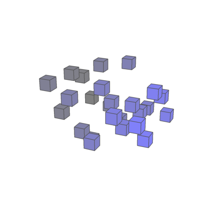
Due a post in the forum I expanded plotcubes() a little bit. It works now better. But it is still not perfect. For photo realistic scenes, you should use Povray via EMT.
>function p (M) ...
 clg;
 plotcubes(M,rgb(0.5,0.5,linspace(0.5,1,rows(M))));
 endfunction
>n=4;
>x=0:1/n:1; {X,Y}=field(x,x);  ...
 X=flatten(X)'; Y=flatten(Y)'; Z=random(size(X)); ...
 h=1/(2*n); M=X|(X+h)|Y|(Y+h)|Z|(Z+h);
>plot3d({{"p",M}},>own,>user,zoom=4,center=[-0.5,-0.5,-0.5]):
The Ctrl-Z to restore a line became more functionality. It will now remember the 8 last version of this line. A new version is stored whenever the line is executed. Moreover, Ctrl-Y does now undo the restore.