Welcome! This is a first introduction into Euler Math Toolbox (EMT) with lots of links and examples.
In case you are reading the HTML page be aware that it has been exported from a notebook in EMT. The notebook itself is installed with EMT and can be opened using "Open Tutorias and Examples" in the File menu.
You can go down to the next command line with the cursor down key. The command line belonging to this comment is empty.
To enlarge the windows of EMT, you can press Ctrl-Shift-Q. This will use your complete screen for the text and the graphics window. Press the combination again to go back to your favorite layout. The layout is saved for the next session. Pressing Ctrl-Q will enlarge the content of the window. You can also set the font sizes in the Options menu.
You can use Ctrl-G to hide the graphics window. Then you can toggle between graphics and text with the TAB key.
Press the return key to execute the plot command in the following command line.
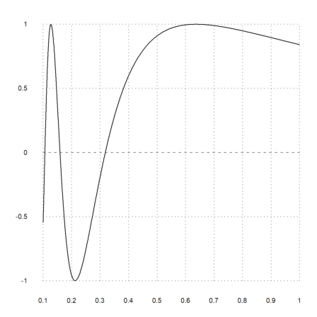
>plot2d("sin(x)*exp(-x^2)",-pi,pi,title="Test",xl="x",yl="y"):
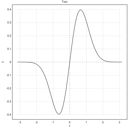
The plot is inserted into the text window by the colon ":" at the end. Plots appear always in the plot window. If you have the plot window hidden by Ctrl-G, press TAB to see the plot now.
Let us first show how to use EMT as a very advanced calculator.
EMT is command line oriented. It allows one or more commands in one command line. The commands have to be ended by a comma or a semicolon.
In the following example, we define a variable r. The output of this definition would be the value of the variable. But because of the semicolon this output is not printed. But the results of the two computations are printed.
>r=1.25; pi*r^2, 2*pi*r
4.90873852123
7.85398163397
We can also concatenate the result with text for an explanation. We will soon learn more refined ways to print numbers.
>"Area = "+(pi*r^2), "Circumference = "+(2*pi*r)
Area = 4.90873852123
Circumference = 7.85398163397
Some remarks on the syntax.
The command r=1.25 is an assignment to a variable in EMT. You can also write r:=1.25 if you prefer. You can leave spaces as you like.
You can also end a command line with a comment.
>r := 1.25 // Comment: You can use := instead of =
1.25
Functions are called with round brackets.
>sin(45°), log(sqrt(E))
0.707106781187
0.5
As you see, trigonometric functions work with radians, and degrees can be converted with °. If your keyboard does not have the degree character press F7, or use the function deg() to convert.
EMT knows a great lot of mathematical functions and operators. For details see
Full Reference
Core Functions
Special Functions
To make chains of computations easier, you can refer to the previous result with "%". It is good style to use this only within the same command line.
>(sqrt(5)+1)/2, %^2-%+1 // Check the solution of x^2-x+1=2
1.61803398875
2
If you want to reuse a result over several lines it is better to use a variable.
>x=(sqrt(5)+1)/2
1.61803398875
>x^2-x+1
2
EMT can convert units to the international standard system (IS). Append the unit to the number for a simple conversion.
>3.56miles
5729.26464
A list of available units can be found on the page below.
For the conversion to and between units, EMT has a special operator -> which can convert to a number or to a string.
>4km -> miles, 4inch -> " mm"
2.48548476895
101.6 mm
The default output format prints with around 10 places. Other output formats can be set globally or only for one output.
For short, long, or longest output of a single value, you can use the following operators.
>short 1200*1.03^10, long E, longest pi
1612.7
2.71828182846
      3.141592653589793
You can switch the output format for all subsequent commands. Reset the format with "defformat" or "reset".
>longestformat; pi, defformat;
3.141592653589793
The numerical kernel of EMT works with floats in double IEEE precision (in contrast to the symbolic part of EMT). But numerical results can be converted to fractions for the output.
>1/7+1/4, fraction %
0.392857142857
11/28
It is possible to print a precise number of decimals. The first way is to set a specific format.
>format(10,2); 1278.89*1.19, defformat;
1521.88
Then there is the print function.
>print(pi,5,10)
3.14159
For C scholars there is also a simple version of printf().
>printf("pi = %10g",pi)
pi = 3.14159
A multi-line command stretches over several lines connected with "..." at the end. To generate such a break in a line, use Ctrl-Return. In the middle of a line, it will make two lines of the line and append "..." to the first part. To revert the split and join a line to the previous line, use "Ctrl-Backspace".
The following multi-line command can be executed whenever the cursor is in any of its lines. It also shows that the ... must be at the very end of the line even if it contains a comment.
>a=4; b=15; c=2; // solve a*x^2+b*x+c=0 manually ...
 diskr=sqrt(b^2/(a^2*4)-c/a); ...
 -b/(2*a) + diskr, ...
 -b/(2*a) - diskr
-0.138444501319
-3.61155549868
Instead of using mutli-line commands, you can also press Shift-Enter to re-run all commands in the current section. Sections are separated by headings or empty lines.
Comments can be entered in front of any command line. To edit the comment, press F5 or simply right click on the comment.
Comments consists of lines, separated by newline commands. Each line is broken into a paragraph in the EMT window. The lines are also broken in the comment editor automatically. It is recommended to use two newline comments to separate paragraphs, as well as after a heading.
For more information about the syntax of comments, press F1 to get help and open the help section about "Comments".
>//
To see all variables that you have defined use "listvar".
>listvar
r                   1.25
x                   1.61803398874989
a                   4
b                   15
c                   2
diskr               1.73655549868123
This searches for the user defined variables only. It is possible to search for other variables. For this, a string should be added which should be contained in the name of the variable.
The following finds all units ending with "m" by searching for all variables that contain "m$".
>listvar m$
km$                 1000
cm$                 0.01
mm$                 0.001
nm$                 1853.24496
gram$               0.001
m$                  1
hquantum$           6.62606957e-34
atm$                101325
To remove a variable without having to restart EMT use "remvalue".
>remvalue a,b,c,diskr
Restarting EMT happens by default if a notebook is loaded (Ctrl-O) or an new empty notebook is created (Ctrl-N). This resets EMT into the starting state.
To get help on any function in EMT, open the help window by F1 and search for the function. You can also double click on a function in the notebook window to open the help window.
Try double clicking on "intrandom" in the following command!
>intrandom(10,6)
[3, 4, 4, 6, 2, 6, 1, 6, 1, 3]
In the help window, you can click on any word to find references or functions.
E.g., try to click on the word "random" in the help window. The word can be in the text or in the "See:" part of the help. You will find that the function "random" creates uniform numbers uniformly between 0.0 and 1.0. From the help for "random" you can walk to "normal" etc.
>random(10)
[0.52143,  0.428893,  0.168134,  0.182742,  0.288048,  0.750042,
0.472935,  0.324407,  0.340388,  0.195494]
>normal(10)
[-0.277172,  -1.4568,  0.658046,  1.53204,  -2.47296,  -0.937381,
0.836566,  -0.233827,  0.221796,  -0.541047]
EMT is a "matrix language". I.e., it uses vectors and matrices for advanced computations. To learn all about this open the following tutorial.
A vector can be defined by square brackets.
>[4,5,6,3,2,1]
[4, 5, 6, 3, 2, 1]
Matrices are available too. In fact, EMT has very advanced features to do Linear Algebra, Statistics or Optimization.
For an example, we can define a vector of uniformly spaced values like the following, and compute the mean of the squared values.
>0:0.1:1, mean(%^2)
[0,  0.1,  0.2,  0.3,  0.4,  0.5,  0.6,  0.7,  0.8,  0.9,  1]
0.35
EMT can use complex numbers too. Many functions work for complex numbers as expected.
>exp(2+3*I)
-7.31511+1.04274i
However, EMT tries to keep the results real and will not automatically switch to complex numbers.
Thus sqrt(-1) will yield an error, but the complex square root is defined for the slit plane in the usual way. To make a real number complex you can add 0i simply or use the fullowing function.
>complex(-1), sqrt(%)
-1+0i
0+1i
EMT does symbolic math with the help of Maxima. For details, start with the following tutorial, or browse the reference for Maxima.
Tutorial on Symbolic Math with Euler
Maxima Reference
Experts in Maxima need to know that there are differences in the syntax between the original syntax of Maxima and the syntax of symbolic expressions in EMT which we call "compatibility mode". The reason for this adaptation is to make Maxima easier to learn for users of EMT and similar numerical systems.
Symbolic math is integrated seamlessly into Euler with the ampersand "&". Any expression starting with "&" is a symbolic expression. It is evaluated and printed by Maxima.
>&expand((1+x)^4), &factor(diff(%,x))
                       4      3      2
                      x  + 4 x  + 6 x  + 4 x + 1


                                       3
                              4 (x + 1)
Again, % refers to the previous result.
A direct input of Maxima commands is available too. Start the command line with "::". The syntax of Maxima is adapted to the syntax of EMT (called the "compatibility mode").
>:: factor(20!)
                        18  8  4  2
                       2   3  5  7  11 13 17 19
If you are an expert in Maxima, you may wish to use the original syntax of Maxima. You can do this with ":::".
>::: av:g$ av^2;
                                   2
                                  g
The same line is much closer to the syntax of EMT in the compatibility mode. One important point is to use ":=" to assign variables only, not the relaxed "=" that is possible in EMT.
>:: av:=g; av^2
                                   2
                                  g
Variables can be stored as symbolic variables using the assignment "&=".
>fx &= x^3*exp(x)
                                 3  x
                                x  E
Such variables can be used in other symbolic expressions. Note, that in the following command the right hand side of &= is evaluated before the assignment to Fx.
>Fx &= integrate(fx,x)
                         3      2             x
                       (x  - 3 x  + 6 x - 6) E
For the evaluation of an expression with specific values of the variables, you can use the "with" operator (an extension of the original syntax of Maxima).
The following command line also demonstrates that Maxima can evaluate an expression numerically with float().
>&(Fx with x=10)-(Fx with x=5), &float(%)
                                10       5
                           754 E   - 74 E


                         1.659697263551068e+7
The most elementary way to define a simple function is to store its formula in a symbolic or numerical expression. If the main variable is x, the expression can be evaluated just like a function.
As you see in the following example, global variables are visible during the evaluation.
>fx &= x^3-a*x;  ...
 a=1.2; fx(0.5)
-0.475
All other variables in the expression can be specified in the evaluation using an assigned parameter.
>fx(0.5,a=1.1)
-0.425
An expression is not necessarily symbolic. Often, symbolic expressions would not work, e.g., if the expression contains functions, which are only known in the numerical kernel, not in Maxima.
>fx="gammai(x^2,2)*cos(x)"; fx(0.5)
0.0232550788778
Technically, expressions are simply strings in EMT. A symbolic expression has an additional flag so that it is automatically printed by Maxima as a Maxima expression. Otherwise, it is a simple string.
>expr &= x^3+x+2; expr,
                               3
                              x  + x + 2
To demonstrate that this is a string, we concatenate with another simple string in EMT.
>"Expression : " + expr
Expression : x^3+x+2
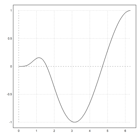
The easiest way to plot a function is to use an expression in x. This can be a symbolic expression or a simple string. We demonstrate more advanced plots later.
In the following example, we also demonstrate that a colon ":" at the end of the command line inserts the current plot into the notebook. By default, the plot is visible in a separate window only. (EMT can also use a one-window interface - press Ctrl-G).
Press TAB to bring the plot window or the plot area to the front.
>plot2d(fx,0,2pi):
In this crash course, we will only show one-line functions. For multi-line functions refer to the following tutorial. EMT contains a complete programming language.
A one-line function can be numerical or symbolic.
>function f(x) &= x^3-x
                                 3
                                x  - x
With &= the function is symbolic, and can be used in other symbolic expressions.
>&integrate(f(x),x)
                                4    2
                               x    x
                               -- - --
                               4    2
With := the function is numerical. A good example is a numerical integral like
![]()
which can not be evaluated symbolically.
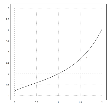
>function f(x) := integrate("x^x",1,x);
A function can be plotted by its name. We add a label "f" to the graph of the function.
>plot2d("f",0,2,-1,3); label("f",1.6,f(1.6)):
Functions can have default values for parameters.
>function mylog (x,base=10) := ln(x)/ln(base);
Now the function can be called with or without a parameter "base".
>mylog(100), mylog(2^6.7,2)
2
6.7
Moreover, it is possible to use assigned parameters.
>mylog(E^2,base=E)
2
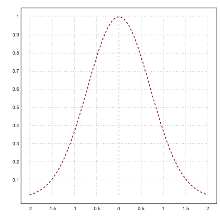
Assigned parameters are used by many functions and algorithms in EMT. E.g., the plot2d function can get parameters in exactly this way.
>plot2d("exp(-x^2)",style="--",color=red,thickness=2):
For boolean parameters, there is a shortcut. The argument ">param" is equivalent to "param=true", and "<param" is equivalent to "param=false". By the way, "false" is defined as 0, and "true" is defined as 1 in EMT. There is no boolean data type.
>plot2d("sin(1/x)",0.1,1,<frame):
There are also purely symbolic functions, which cannot be used numerically.
>function lapl(expr,x,y) &&= diff(expr,x,2)+diff(expr,y,2)
diff(expr, y, 2) + diff(expr, x, 2)
>&realpart((x+I*y)^4), &lapl(%,x,y)
                           4      2  2    4
                          y  - 6 x  y  + x


                                  0
But of course, they can be used in symbolic expressions or in the definition of symbolic functions.
>function f(x,y) &= factor(lapl((x+y^2)^5,x,y))
                          2     3     2
                     10 (y  + x)  (9 y  + x + 2)
To summarize
Equations can be solved numerically and symbolically.
To solve a simple equation of one variable, we can use the solve() function. It needs a start value to start the search. Internally, solve() uses the secant method by default.
>solve("x^2-2",1)
1.41421356237
This works for symbolic expression too. Take the following function.
>px &= 4*x^8+x^7-x^4-x, plot2d(px,-1,1):
                             8    7    4
                          4 x  + x  - x  - x
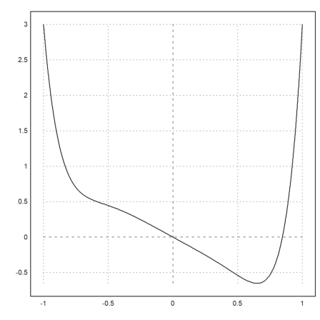
Now we search the point, where the polynomial is 2. In solve(), the default target value y=0 can be changed with an assigned variable. This numerical function requires a start value for the iteration.
We use y=2, a start value of x=1, and check by evaluating the polynomial at the computed solution.
>solve(px,1,y=2), px(%)
0.966715594851
2
Solving a symbolic expression in symbolic form returns a list of solutions. We use the symbolic solver solve() provided by Maxima.
>sol &= solve(x^2-x-1,x)
                       1 - sqrt(5)      sqrt(5) + 1
                  [x = -----------, x = -----------]
                            2                2
The easiest way to get the numerical values is to evaluate the solution numerically just like an expression.
>longest sol()
-0.6180339887498949 1.618033988749895
To use the solutions symbolically in other expressions, the easiest way is "with".
>&x^2 with sol[1], &expand(x^2-x-1 with sol[2])
                                         2
                            (sqrt(5) - 1)
                            --------------
                                  4


                                  0
There are many more functions to solve equations, like the Newton method or the bisection method. Moreover, there are interval methods, which return guaranteed inclusions of the solution.
Reference on Numerical Algorithms
Tutorial on Numerical Analysis
Tutorial on Interval Methods
Solving systems of equations symbolically can be done with vectors of equations and the symbolic solver solve(). The answer is a list of lists of equations.
>&solve([x+y=2,x^3+2*y+x=4],[x,y])
[[x = - 1, y = 3], [x = 1, y = 1], [x = 0, y = 2]]
Solving systems of nonlinear equations numerically requires advanced numerical methods.
In general, a function is required for this. Here is just one short example.
>function f([x,y]) := [sin(x)+y-2,x^3+2*y+x-4];
The Broyden method is a good general method to solve such equations. But there are more methods. See
Newton and Quasi-Newton Methods
The Broyden algorithm does not need the derivative of the function.
>broyden("f",[1,1]), f(%)
[0.870078,  1.23562]
[0,  0]
Like Matlab or NumPy, EMT is a matrix language. It is designed to handle vectors and matrices, im most cases without explicit loops. In this first tutorial, we only show a basic example.
Let us generate a vector of equally spaced numbers.
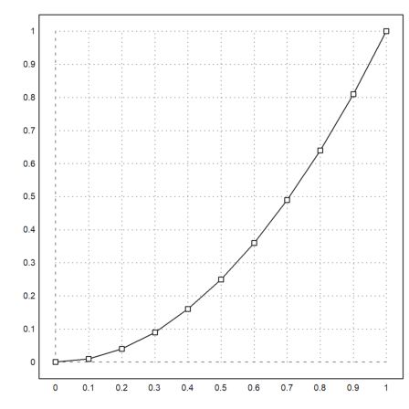
>x = 0:0.1:1
[0, 0.1, 0.2, 0.3, 0.4, 0.5, 0.6, 0.7, 0.8, 0.9, 1]
We can now use x in an expression, and the expression will be evaluated element by element.
>y = x^2
[0, 0.01, 0.04, 0.09, 0.16, 0.25, 0.36, 0.49, 0.64, 0.81, 1]
This can be used in the plot command to plot the points or a line through the points.
>plot2d(x,y,>addpoints):
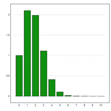
The matrix language works for almost all functions automatically. For an example, we generate the binomial distribution for p=1/3 and plot it using a special plot function for statistics.
>n = 0:10; p = 0.3; ...
 columnsplot(bin(10,n)*p^n*(1-p)^n,lab=n):
Let us also mention that we can use Latex code in EMT comments if Latex is installed.
![]()
This tutorial can only be a starting point. To continue you can study the tutorial on special topics in EMT which are installed with EMT. Or you can press F1 to open the help window and clear the search box with ESC. You will get a list of help topics for EMT to guide you along.
The author wishes you a lot of fun with math and EMT! There is a lot to learn. So keep experimenting. That's what EMT was made for.