Our first example is a simple one-line function. Such a function is defined by the "function" keyword, the function name with variables, a ":=", and an expression.
>function f(x) := x^3+x^2-x
The function can be used in any numerical expression, just like the built-in functions.
>f(5)+f(f(3))
37138
You can also define a symbolic function, which will work in symbolic expressions too. Of course, this is only possible if the function uses a simple expression, and if this expression can be evaluated by Maxima.
>function f(x) &= x^3+x^2-x
                              3    2
                             x  + x  - x
In fact, the evaluation of symbolic expressions takes place at compile time. The right hand side will be evaluated before the function is defined, as you can see in the following example.
>function df(x) &= diff(f(x),x)
                               2
                            3 x  + 2 x - 1
The function will work for vectors x, since the Euler matrix language takes care of matrix values in expressions automatically, and this function uses only a simple expression.
>f(1:10)
[1, 10, 33, 76, 145, 246, 385, 568, 801, 1090]
You can break one-line functions in two lines.
>function f(x) := x^4+x^3+x^2 ...
   +x;
As you see, they will still simply evaluate a single expression.
>type f
function f (x)
useglobal; return x^4+x^3+x^2+x;
endfunction
Note the "useglobal" command which makes all global variables visible. The next three lines show, that one-line functions can also be a part of a multi-line command, if they are closed with a semicolon ";".
>aglob=4;  ...
 function f(x) := aglob*x; ...
 f(5)
20
The same function can also be defined in multiple lines. Then the function definition must end with a line containing "endfunction" The function can contain a return statement, or else it will return the special string value none (string with character 0x01).
To enter such a function, its lines can be entered one by one, until "endfunction" finishes this input mode (press return in an empty line to get "endfunction").
>function f(x)
 return x^3+x^2-x
 endfunction
Alternatively, enter the function line and press Ctrl-Return. This will put you in a special mode to edit a function.
Here is the same multi-line function with ... in the first line. Then the function can be defined in the "function" line when the enter key is pressed.
>function f(x) ...
 return x^3+x^2-x
 endfunction
Another method is to use the internal editor with F9 in the function line.
To edit such a multi-line function click somewhere inside the function and edit the function. Exit this mode with the escape key or with the return key. This is a special mode for editing functions. Some useful keys are
The following function f() defined in the previous section works for real numbers.
>f(2)
10
It also works for complex numbers.
>f(I)
-1-2i
And even for intervals.
>f(~2,3~)
~9,34~
Likewise for vectors.
>f(1:5)
[1, 10, 33, 76, 145]
But not for strings.
>f("test")
Wrong argument.
Cannot use a string here.

Error in ^
Try "trace errors" to inspect local variables after errors.
f:
    return x^3+x^2-x
Error in:
f("test") ...
         ^
To make sure, the function is not abused, we can fix its parameter type as follows.
>function f(x:numerical) := x^3+x^2-x
Now, we get a meaningful error message.
>f("test")
Function f needs a numerical type for x
Error in:
f("test") ...
         ^
There are many more parameter types to help error checking.
You can combine some of these types. Here are some predefined combinations.
You can also do error checking with typeof(...) and error(...).
>function myprint (s, n:index) ...
 if typeof(s)==8 then return printstr(s,n);
 elseif typeof(s)==0 then return printstr(""+round(s,n-5),n);
 else
   error("Cannot print this");
 endfunction
The types are numbers. 8 is for strings.
>myprint("Affe",10)
Affe
A real is of type 0.
>myprint(pi,10)
3.14159
In all other cases we get an error.
>myprint(I,10)
Error : Cannot print this

Error generated by error() command

Try "trace errors" to inspect local variables after errors.
myprint:
    error("Cannot print this");
A multi-line function can contain comment lines starting with ## and a blank. The first comment lines appear in the help command.
>function f(x) ...
 ## Computes x^3-x
 ## Just an example for a comment line.
   return x^3-x
 endfunction
The help command now displays the function, the help, and some additional information.
>help f
f is an Euler function.

function f (x)

Entered from command line.

Computes x^3-x
Just an example for a comment line.
If you place the cursor at after the opening bracket in the following line, the status line will show the parameters of the function and the first comment line.
>f(10)
990
The same works for one-line functions in the following way.
>function f(x) := x^3-x // Compute x^3-x
The following function demonstrates how to return multiple values from a function. (We explain the "if" statement in the next section).
>function ordertwo (a:number, b:number) ...
   if a<b then return {a,b}
   else return {b,a}
   endif;
 endfunction
To assign multiple values, you use the same {...} syntax.
>{a,b}=ordertwo(4,2); [a,b]
[2, 4]
Multiple return values by default do not serve for multiple arguments to another function. Only the first return value is used by default.
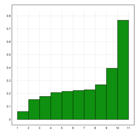
The sort() function returns two values, the sorted vector and the indices of the sorted elements. Only the sorted vector is used in the following call to plot2d.
>plot2d(sort(random(1,10)),>bar):
If a function has the "args" modifier as in
function args histo (v) ...
its multiple returns can be used as parameters in other functions.
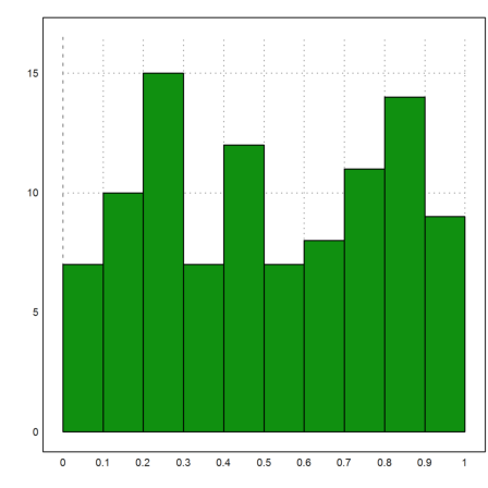
So we can easily use the multiple result of histo(v) to plot a histogram. The function histo(v) returns {x,y} suited for bar plots.
>plot2d(histo(random(1,100),v=0:0.1:1),>bar):
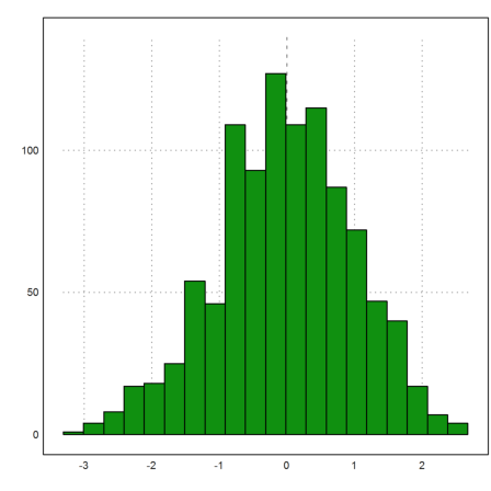
Of course, it might be clearer to assign the result to variables first.
>{x,y}=histo(normal(1,1000),20); plot2d(x,y,>bar):
Multiple returns can also be used to assign two values to two variables simultaneously.
The following version of the Euclid's algorithm makes use of this.
>function mygcd (n:index, m:index) ...
 if n<m then {n,m}={m,n}; endif;
 repeat
   k=mod(n,m);
   if k==0 then return m; endif;
   if k==1 then return 1; endif;
   {n,m}={m,k};
 end;
 endfunction
>mygcd(123456795,1234567851)
33
Of course, there is a built-in function named gcd().
>gcd(123456795,1234567851)
33
The Euler programming language has the usual control statements. Control statements change the flow of execution. Control statements cannot be used in one-line functions.
The loop with a named variable and an optional increment (step ...) is one of them.
>function test ...
 for i=1 to 5; i, end;
 endfunction
>test;
1
2
3
4
5
It should be mentioned that loops work outside of functions in the command line too, as long as the complete loop fits within a single line or a multi-line.
>for i=1 to 5; i, end;
1
2
3
4
5
The "for" loop can have a step value.
>for i=5 to 1 step -1; i, end;
5
4
3
2
1
And it can loop over a vector.
>v=random(1,5); for x=v; x, end;
0.653846096982
0.437003931098
0.16401194918
0.888343651085
0.688567028627
The following function definition does the same with "repeat".
>function test ...
 n=1;
 repeat
   n,
   n=n+1;
   if n>5 then break; endif
 end
 endfunction
"repeat" is an infinite loop. It can be aborted with the "break" command, which jumps to the first command after the end of the loop. We put the "break" into an "if" clause, testing for n>5.
Note, that each "if" clause must end with "endif". On the other hand, loops end with "end".
>test;
1
2
3
4
5
Instead of the "break" inside the conditional statement, Euler has "until" and "while". Both statements must be inside a "repeat" loop. The loop must still end with "end".
>function test ...
   n=1;
   repeat
     n, n=n+1;
     until n>5;
   end
 endfunction
The "while" statement reverses the condition.
>function test ...
   n=1;
   repeat while n<=5;
     n, n=n+1;
   end
 endfunction
>test
1
2
3
4
5
Here is a definition of the modulus function, using an else clause. Of course, it is already contained in Euler as "abs".
>function test (x:number) ...
 if x<0 then return -x; else return x; endif
 endfunction
>test(-1), test(1),
1
1
If can also have one or more "elseif" clauses. So you do not need to put one "if" inside the other.
>function test (x:number) ...
   if x>0 then "positive",
   elseif x<0 then "negative",
   else "zero",
   endif;
 endfunction
>test(-1), test(0), test(1),
negative
zero
positive
The function in the previous example would not work for vectors! We have made the function type safe by requiring x to be a scalar with the "number" keyword.
To make the function work for vectors and matrices too, we can either map it at runtime, or define the function with the "map" keyword.
At runtime, the function can be forced to map by appending "map" to the function name.
>testmap(-1:1)
negative
zero
positive
At compile time, we use "function map ...".
The following example returns the absolute value of a number. (Of course, there is a function "abs" in Euler already.)
>function map test (x) ...
 if x<0 then return -x; else return x; endif
 endfunction
>test(-1:1)
[1, 0, 1]
It is possible to prevent mapping using a semicolon in the parameter list when the function is defined.
In the following example, we do not want to map to the coefficients of the polynomial p.
>function map test (x; p) := evalpoly(x,p)
The function maps only to the first argument. We evaluate
![]()
in the following example.
>test(0:0.2:1,[1,2,1])
[1, 1.44, 1.96, 2.56, 3.24, 4]
By the way, the function evalpoly() is already defined in EMT.
>evalpoly(0:0.2:1,[1,2,1])
[1, 1.44, 1.96, 2.56, 3.24, 4]
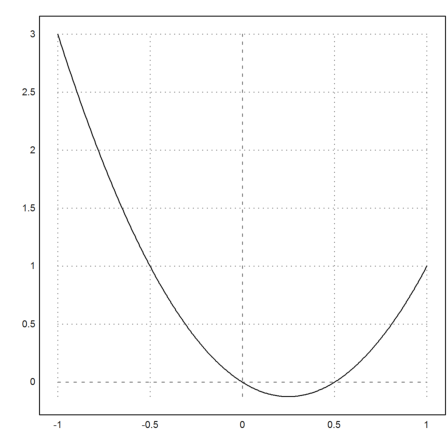
For another example, we implement
![]()
>function map f(x;a) := sum(abs(x-a));
Then f(a,a) will work for a vector a, since it computes f(x,a) for all x in the vector a.
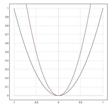
>a=1:10; plot2d("f(x,a)",1,10); plot2d(a,f(a,a),>points,>add):
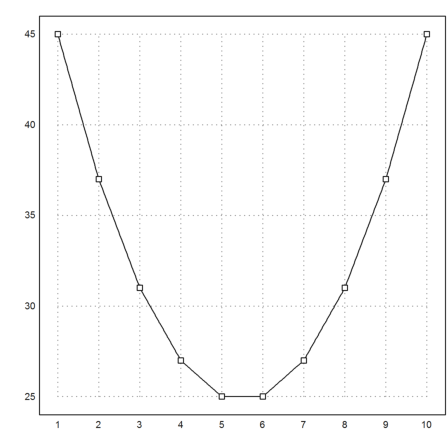
One should remark here that the same can be achieved for two vectors x and a with the matrix language of EMT in the following way.
>sum(abs(a'-a))', f(a,a)
[45,  37,  31,  27,  25,  25,  27,  31,  37,  45]
[45,  37,  31,  27,  25,  25,  27,  31,  37,  45]
You should not do your own vectorization with loops, but it can be done.
A matrix element A{i} is just the i-th element of the flattened matrix. For a scalar, it will return the scalar value. The size() function returns the proper size of the result.
>function ts (v,w) ...
 s=size(v,w); res=zeros(s);
 loop 1 to prod(s)
    res{#}=v{#}*w{#};
 end;
 return res
 endfunction
This will work in almost all cases.
>ts([1,2;3,4],6)
            6            12
           18            24
But it will fail for a matrix and vector. For this, you can simply use v*w.
>[1,2;3,4]*[5,6]
            5            12
           15            24
By default, functions cannot see global variables. The command "useglobal" inside a function, however, makes all global variables visible. This command is inserted automatically for one-line functions.
>function f(x) := a*x
We can type the internal commands of a function using "type".
>type f
function f (x)
useglobal; return a*x
endfunction
The function can access global variables.
>a:=55; f(2)
110
In a multi-line function, a global variable, or several global variables, can be selected.
>function f(x) ...
 global a;
 return a*x;
 endfunction
A global variable can also be set to be visible in all functions.
>aglob=55; setglobal aglob;
>function f(x) ...
 return aglob*x
 endfunction
The variable "aglob" is found, even though there is no "useglobal" or "global" command.
>f(2)
110
Using global variables is not a good programming style. It is better to pass the variable as an argument to the function.
>function f(x,a) := a*x
>f(2,55)
110
Variables ending with $ are automatically global. All units are defined like this.
>function toinch(x) ...
 return x/inch$
 endfunction
>toinch(1.56ft)
18.72
Global variables are mutable. To generate a global variable inside a function, use the "global" statement with an assignment (or end the variable name $$).
>function test1 () ...
 global a = 1:8;
 endfunction
To access an existing global variable, use the "global" statement with the name of this variable.
>function test2 () ...
 global a;
 return 2*a
 endfunction
>test1; test2,
[2, 4, 6, 8, 10, 12, 14, 16]
Note, that pi() is a built-in function. But you can use it like a global variable everywhere, because EMT looks for functions with no arguments if it does not find a variable.
>1.2^2*pi
4.52389342117
In EMT, you can provide default values for parameters. The following function computes norms of a row vector.
>function pnorm (v:vector, p:nonnegative number=0) ...
   if p>=1 then return sum(abs(v)^p)^(1/p);
   else return max(abs(v))
   endif;
 endfunction
If p=0 (the default), pnorm() computes the maximum norm.
>v=[2,3,-2]; pnorm(v)
3
Or the Euclidean norm for p=2.
>pnorm(v,2)
4.12310562562
Default parameters can also be set by name.
>pnorm(v,p=1)
7
To prevent typos, named arguments can only be used for parameters with default values. You will get an error if you try to use a name which is not in the list of default parameters.
>pnorm(v,pp=1)
Argument pp not in parameter list of function pnorm.

Parameters:
v, p

Error in:
pnorm(v,pp=1) ...
             ^
However, a new variable can be created in the function with ":=".
>function f(x) := x*a; ...
 f(5,a:=6)
30
If the function has the modifier "allowassigned", other assigned arguments can be used than are in the parameter list, even if they are not defined by ":=".
>function allowassigned f(x) := x*a; ...
 f(4,a=7)
28
A frequent way to use a default parameter is with the default value "none". This is done in many Euler functions to be able to check, if the user has set this parameter or not.
>function multmod (a:integer, b:integer, p:index=none) ...
   if p==none return a*b
   else return mod(a*b,p)
   endif;
 endfunction
>multmod(7,9)
63
>multmod(7,9,11)
8
As an example, we take the following function to cook eggs. I found the formula in a book by Werner Gruber.
![]()
The diameter of the egg is in millimeters, the temperatures in Celsius, and the result is in minutes. We provide good default values for the parameters. The water will be close to 95°, an egg from the refrigerator should be around 6°, and for a soft-boiled egg we want 62°.
>function tegg(d,tw=95,ts=6,ti=62) := 0.0016*d^2*log(2*(tw-ts)/(tw-ti))
As an example, we compute the times in minutes for eggs from 40mm to 50mm.
>de=(40:50)'; te=tegg(de)
      4.31431
      4.53272
      4.75652
      4.98572
      5.22031
      5.46029
      5.70567
      5.95644
       6.2126
      6.47416
       6.7411
Now we compute the minutes and the seconds, and print with writetable().
>tem=floor(te); tes=round((te-tem)*60); ...
 writetable(de|tem|tes,labc=["d","min","sec"])
         d       min       sec
        40         4        19
        41         4        32
        42         4        45
        43         4        59
        44         5        13
        45         5        28
        46         5        42
        47         5        57
        48         6        13
        49         6        28
        50         6        44
We might give the user some constants so that values for parameters can be easily remembered.
>softegg=62; hardegg=82; fridge=6; room=20; ...
 writetable(tegg(45,ts=[fridge,room],ti=[softegg,hardegg]'), ...
    labc=["fridge","room"],labr=["soft","hard"])
              fridge      room
      soft      5.46      4.91
      hard      8.48      7.92
Scalar arguments work as if they are passed to functions by value. If you change the value, it will not change the value of the variable passed to the function.
>function f(x) ...
   x=4;
 endfunction
In the following example, a is not changed.
>a=5; f(a); a,
5
Of course, the name of the parameter inside the function does not matter at all. It is a local name.
>x=5; f(x); x,
5
To allow passing an argument by reference, the parameter name must start with %... Even in this case, only the value of the parameter can be changed, not its size or type.
>function f(%x) ...
   %x=4;
 endfunction
>x=5; f(x); x,
4
>x=I; f(x); x,
Cannot change type of non-local variable x!
Try "trace errors" to inspect local variables after errors.
f:
    %x=4;
Vectors and matrices work as if they are passed by reference. So a function can change the elements of the vector or matrix.
>function f(x) ...
   x[1]=5;
 endfunction
>x=1:10; f(x); x,
[5, 2, 3, 4, 5, 6, 7, 8, 9, 10]
If you do not want this, you need to make a local copy. Even a copy to a variable with the same name will work.
>function f(x) ...
   x=x;
   x[1]=5;
   return x;
 endfunction
>x=1:10; f(x), x,
[5,  2,  3,  4,  5,  6,  7,  8,  9,  10]
[1,  2,  3,  4,  5,  6,  7,  8,  9,  10]
It is only possible to change elements of the vector or matrix, not the complete global matrix.
If you want to change a matrix in the calling program or globally, you must return the matrix from the function and assign the returned value.
>function f(x) ...
   y=x;
   y[1]=2;
   return y;
 endfunction
>x=f(x); x,
[2, 2, 3, 4, 5, 6, 7, 8, 9, 10]
Of course, you can always define a mutable global variable.
>function test() ...
 global M = [1,2;3,4];
 endfunction
Such variables can be used and changed everywhere in the program, globally or in another function.
>test; M[2,2]
4
In one-line functions, the symbolic expression is evaluated at compile time.
>function f(x) &= diff(x^x,x)
                            x
                           x  (log(x) + 1)
The same is possible in multi-line functions. The syntax for this is &:"...".
>function f(x) ...
   return x+&:"diff(x*exp(x),x)"
 endfunction
As you see, the function is indeed defined using the evaluated expression.
>type f
function f (x)
return x+x*E^x+E^x
endfunction
Note that the string returned by Maxima is inserted verbatim. You may want to user brackets in some cases.
It is also possible to call Maxima at run time in functions. The syntax is &"...". Note that this will slow down your function considerably.
However, with run time calls it is possible to include the value of a parameter into the Maxima command using the @... syntax.
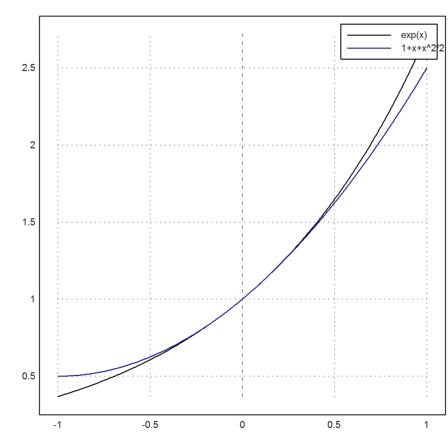
>function drawtaylor (expr,a,b,n) ...
   plot2d(expr,a,b);
   dexpr = &"taylor(@expr,x,0,@n)";
   plot2d(dexpr,>add,color=blue,>add);
   labelbox([expr,dexpr],colors=[black,blue]);
 endfunction
>drawtaylor("exp(x)",-1,1,2):
Sometimes you need an expression, evaluated at compile time, inside a string.
>function map f(a) := integrate("&:taylor(x^x,x,1,2)",1,a)
>type f
function map f (a)
useglobal; return integrate("1+(x-1)+(x-1)^2",1,a)
endfunction
This function defines
![]()
with the Taylor polynomial of degree 2 of x^x around 1
![]()
>plot2d("f",0.5,1.5):
A function can call itself. So we can also program recursively in EMT. Of course, we have to make sure the recursion is not infinite. Moreover, there is a limit for the number of recursions.
In the following definition of the factorial function, we use a "return" inside an if clause to stop the recursion.
>function fact (n:natural) ...
   if n<=0 then return 1; endif;
   return n*fact(n-1)
 endfunction
This defines the factorial function.
>fact(5)
120
We can achieve the same result with a loop. In the following definition, we use a simple integer loop. The loop index can be accessed with "#".
>function map fact1 (n:natural) ...
   x=1; loop 2 to n; x=x*#; end;
   return x;
 endfunction
This should be a bit faster.
Since we used the keyword "map", it will also work for vector input.
>fact1(1:5)
[1, 2, 6, 24, 120]
The matrix language of EMT has a better solution for this.
>cumprod(1:5)
[1, 2, 6, 24, 120]
Let us try to evaluate the Chebyshev polynomial of degree n at x, using the recursive formula
![]()
Of course, EMT has the much more efficient function cheb() already, but we want to demonstrate the program here.
We could use a recursive definition, but is far more effective to make it in a loop.
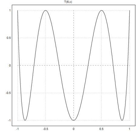
>function t (n:natural, x:vector) ...
   if n==0 then return ones(size(x)); endif;
   if n==1 then return x; endif;
   a=1; b=x;
   loop 2 to n;
     {a,b}={b,2*x*b-a};
   end;
   return b
 endfunction
The function works for vectors x, even if n=0. It does not work for vectors n.
>x=-1:0.01:1; plot2d("t(6,x)",title="T(6,x)",a=-1,b=1):
By the way, it is surprising how accurate the formula is. This is due to a cancellation of errors.
>longformat; t(60,0.9), cos(60*acos(0.9)),
-0.350468376614
-0.350468376614
Let us try to get the Chebyshev polynomial itself. We have to struggle with the vectors containing the coefficients of the polynomial.
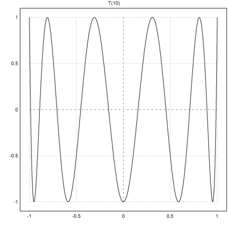
>function T (n:natural) ...
   if n<=0 then return [1]; endif;
   if n==1 then return [0,1]; endif;
   a=[1]; b=[0,1];
   loop 2 to n;
     c=[0,2*b]-[a,0,0];
     a=b; b=c;
   end;
   return b
 endfunction
Now T(n) returns the coefficients of the n-th Chebyshev polynomial.
>T(4)
[1, 0, -8, 0, 8]
We can evaluate a polynomial with "evalpoly".
>plot2d("evalpoly(x,T(10))",title="T(10)",a=-1,b=1):
However, this is not an accurate procedure for large n. (Compare with the result above).
>p=T(60); evalpoly(0.9,p)
-14447.2139393
Though it is not efficient either, we can use an accurate solver for the evaluation of this polynomial. We see that the reason of the inaccuracy is the Horner scheme.
>xevalpoly(0.9,p)
-0.350468376613
Euler contains a very accurate evaluation of the Chebyshev polynomials.
>cheb(0.9,60)
-0.350468376614
Some functions require a vector input and output. But we might want to use variable names for the vector elements. Euler can use the following syntax for this.
>function f([x,y]) := [x*y-1,x-y]
The Broyden algorithm can solve systems of n equations with n unknowns. It expects a function f(v) mapping a vector to a vector.
For an example, we find the solution of x*y-1=0 and x-y=0.
>broyden("f",[1,0])
[1, 1]
The function f will work for column vectors, and for single elements, if these elements are scalar.
>f(1,1)
[0, 0]
>f([1,1])
[0, 0]
Many algorithms of Euler can use a function or an expression as parameters. Such functions accept the function or expression in a string, and then evaluate it like a normal function or expression.
To program such an algorithm, you should name the function parameter ending with $. It is not possible to define a function with such a name, so there is never a name conflict. This is a good practice because internal and DLL functions take precedence over parameter functions.
>function test (f$:string,x) := f$(x)
The string f$ can now be used for any function, including built-in functions.
>test("sin",pi/2)
1
It can also be used for expressions.
>test("x^2",2)
4
The reason for this is, that an expression "expr" using the variable x can be evaluated by "expr(value)".
The evaluation of a string in the function test() can see global variables.
>a:=5; test("x^2+a",2)
9
If a function or an expression passed by a string needs additional arguments, you can pass these arguments as semicolon arguments. Let us demonstrate a function first.
>function f(x,a) := a*x^2
>function test(f$:call,x) := f$(x,args())
Note the parameter type "function". This is either a function name or an expression (or a list, see below).
Now we want to evaluate "f" with a=4 at the point 3.
>test("f",3;4)
36
Here, the value 4 is passed as an additional argument to f by test().
The plot2d and other functions use the same trick to pass arguments to functions.
>plot2d("f",-1,1;1); plot2d("f";2,color=red,>add):
It is also possible and cleaner to use a list with the function name and the additional parameters. E.g., for a=4 we can use the following list. The parameter type "function" lets f$ accept list arguments if the first element of the list is a string.
>test({{"f",4}},3)
36
This works with many numerical functions too.
>bisect({{"f",4}},1,2,5), f(%,4)
1.11803398875
5
For expressions, this is only necessary for local variables, since expressions can see global variables.
>function g(x,a) ...
   return test("a*x^2",x;a)
 endfunction
Without the ";a", the evaluation would use the global value of the variable a.
>g(2,5)
20
In the numerical functions of EMT, you have to use call collections.
>function F(x,a) := integrate({{"1/(1+x^a)",a}},0,x); ...
 F(1,3), integrate("1/(1+x^3)",0,1)
0.888313572652
0.835648848265
Note that the function args() (used in test(f$,x) above) can return multiple results, which will all be used as arguments.
>function f(x,a,b) := a*x+b*x^2
We can plot
![]()
now, setting a=-1 and b=2 with semicolon parameters for f.
>plot2d("f",-1,1;-1,2):
It is recommended to save functions in Euler files. These files have the extension ".e", and should be located in the directory of the notebook.
The following is a test file I made for this example. You can edit the file by pressing F9 or F10 in the next line. However, you might not be able to save your changes, since you cannot write to the installation directory.
>load test
This comment prints, when the file is loaded.
It loads the comment section of the Euler file. Here is the content of the file.
So to make a script file for EMT, you type a line "load filename" into the notebook and press F9. If the script file does not exist it will be generated by EMT in the current directory (the directory of the notebook).
>printfile("test.e")
// * Test File

comment
This comment prints, when the file is loaded.
endcomment

// This is a paragraph of text for the HTML export

// * Section I

// Another paragraph of text.

function test (x)
## Just a test function, prints x.
    return "You entered the argument "+x;
endfunction

function testf (y) := y^y

testvar := 5; // test variable
The functions in the file are now defined in Euler.
>test(23)
You entered the argument 23
The help for test will work too, including the help in the status line.
>help test
test is an Euler function.

function test (x)

Function in file : test

Just a test function, prints x.
Also the variables defined in the file exist in Euler.
>testvar
5
You can export an Euler file to HTML with a menu entry in the File menu. To link to the HTML export use either of the following forms of links.
The user can double click on the link.
Euler files can call each other. Make sure, that no Euler file calls itself recursively.
Euler has a somewhat limited support for operators. There are infix, prefix, and postfix operators. The names of operators have the same restrictions as the names of functions. You cannot define symbols as operators.
As a first example we define the operator pf for fractional print of a number.
>function prefix pf (x) := frac(x)
Then you can call the function pf without round brackets.
>pf 1/6+1/7
13/42
The predefined function fraction does this in a similar way. However, it can also print matrices.
>fraction inv([1,2;3,4])
       -2         1
      3/2      -1/2
As you see, the operator pf binds weakly. By internal reasons, it is not possible to define a strong prefix operator. But for infix and postfix operators, this is possible.
The following operator will bind strong. Note that it overwrites the internal function mod. So we must call this internal function as _mod, and enable the overwrite flag.
>function overwrite strong operator mod (x:integer, n:index) := _mod(x,n)
Note that now the operator mod is evaluated before the + operator.
>11 mod 7 + 12 mod 7
9
It might be more practical to define a weak postfix operator for a specific prime.
>function postfix mod7 (x:integer) := _mod(x,7)
>11+12 mod7
2
Parameter of Euler functions can be anonymous. If a function has no parameter, it can be called with a variable number of parameters. The parameters can be accessed with
 argn(): Number of arguments
 arg1,args2,...: Individual arguments
 getarg(n): Argument number n
 args(n): Arguments starting with the n-th argument
>function sumx () ...
 res=0;
 loop 1 to argn();
   res=res+getarg(#);
 end;
 return res
 endfunction
>sumx(1,2,3,4,5)
15
For a recursive version, you will need args(n).
>function sumx () ...
 if argn()==0 then return 0;
 else return arg1+sumx(args(2));
 endif;
 endfunction
>sumx(1,2,3,4,5)
15
You can mix this style with valued parameters only if you use argument variables.
>function f() := a*arg1; ...
 f(6,a:=7)
42
Since Euler checks the number of parameters for all function with at least one argument, you need to tell Euler that your function has additional arguments. Use the eclipse sign ",...)" or ", ...)" for this.
>function printnumbers (format:string,...) ...
 loop 2 to argn();
   printf(format,getarg(#)),
 end;
 endfunction
>printnumbers("%5.2f",1,2,pi)
 1.00
 2.00
 3.14
In most cases, you can just as well use a vector. Or you can map the printing to the elements of a vector.
>function map printnumbers (v,format) ...
 printf(format,v),
 endfunction
>printnumbers([1,2,pi],"%5.2f")
 1.00
 2.00
 3.14
We did not protect the format from mapping. Thus the function works also in the following way.
>printnumbers(pi,["%10.2f","%10.2e","%10g"])
      3.14
 3.14e+000
   3.14159
Built-in functions and user defined functions can have an alias.
>alias sinus sin;
The alias can be used like any other function.
>sinus(pi/2)
1
EMT has a tracing command. In this state a command runs step by step. In each step, variables can be inspected or expressions can be evaluated using the local variables.
The following can trace commands are available.
  trace on - trace always
  trace off - stop tracing
  trace function - trace inside this function only
  trace alloff - stop tracing specific functions
In the tracing mode, use the following keys.
  cursor-down : single step
  cursor-right : do not trace called functions
  cursor-up : run until return
  cursor-left : stop tracing
  insert : evaluate an expression.
There is also
traceif condition - start tracing if the condition is true
In the following command, tracing will start, if x gets large.
>function f(x) ...
 repeat
    xnew=1+x^2/5;
    until x~=xnew;
    traceif abs(x)>1000;
    x=xnew;
 end;
 return xnew;
 endfunction
If all goes well it converges to the solution of
![]()
>f(2)
1.38196601125
But with the wrong starting point, this will not work. Try the following after un-commenting the command.
>// f(20)
It is possible to let programs stop on errors. There you can inspect the local variables of the function. To start this mode, enter
trace errors
Euler can fold commands and function, so that only the first line is visible.
Function can start with
>function ... // normal function
>%% function ... // hidden function
>%+ function ... // forced folded function
You should start a function definition like this. Anything else may work, but it will confuse the notebook editor.
>%+ function forcedfolded () ...
 ## This will fold away, if it hasn't the focus.
 return "Test"
 endfunction
Functions can also be folded with Ctrl+L just like multi-line commands.
Put the focus elsewhere and press Ctrl+L to see this.
>function canbefolded ()  ...
 ## This can be folded away with Ctrl+L
 return "Test"
 endfunction