This notebook introduces the Fast Fourier Transform (FFT). We will use it to analyze a WAV file.
Mathematically, the FFT evaluates a polynomial in all complex n-th roots of unity simultaneously. If n is a power of 2 (or has at least not many prime large prime factors) the algorithm is very fast.
To demonstrate this, we set xi equal to all 8-th roots of unity.
>xi=exp(I*2*Pi/8); z=xi^(0:7);  ...
   plot2d(re(z),im(z),points=1):
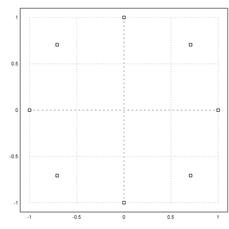
These are the complex values
![]()
for n=8, k=0,...8.
For a test, we generate a complex polynomial of degree 7. We take a random polynomial.
>p=random(1,8)+1i*random(1,8);
We evaluate this polynomial at all points of z. Note that a polynomial is represented in EMT in a vector starting with the lowest coefficient.
>longestformat; evalpoly(z,p)
[ 3.61513775646999+4.027250420449434i,
-0.06067706070439005+0.8797662696327804i,
0.1325483481709888-0.1451728061492038i,
-0.0005680160112071508-0.9346386176109833i,
1.422171838062166-1.867849911920374i,
0.3965191106395581+0.1482400937388588i,
-0.4481910174229353-0.0126947295288784i,
0.1863898275842544+0.1666181435935085i ]
This is exactly the same as FFT of p.
>max(abs(fft(p)-evalpoly(z,p)))
1.799837261104273e-015
The inverse of an evaluation is interpolation. Thus the inverse operation to fft() interpolates values in the roots of unity with a polynomial of degree n. The result contains the coefficients of the interpolating polynomial.
The inverse of fft() is ifft() in EMT. We can go back and forth.
>short ifft(fft(p))-p
[ 0+0i , 0+0i , 0+0i , 0+0i , 0+0i , 0+0i , 0+0i , 0+0i ]
The inverse FFT is almost the same as the original FFT. The operation involves two conjugations and the factor n.
>max(abs(8*conj(ifft(conj(p)))-fft(p)))
0
For those interested in the mathematics, we can write b=fft(a) as
![]()
From this,
![]()
because the last sums are 0, if j is not equal to k.
FFT can also be used to evaluate a trigonometric series at equidistant points.
![]()
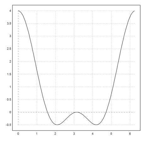
Let us take a cosine series
![]()
and evaluate it directly. Our series has only three terms.
>t=(0:127)*2*Pi/128; s=1+2*cos(t)+cos(2*t); plot2d(t,s):
Now we evaluate it with FFT.
![]()
This is very much faster. For the FFT, we must set the rest of the coefficients to 0.
>a=zeros(1,128); a[1:3]=[1,2,1]; totalmax(abs(re(fft(a))-s))
1.776356839400251e-015
For another example, we evaluate
![]()
for n=1024 in n equidistant points.
>n=1024; d=2*pi/n; plot2d((0:n-1)*d,im(fft(0|1/(1:n-1)))):
FFT and its inverse operation can be used to determine frequencies in a signal. The reason for this is that the functions
![]()
are orthogonal, and the interpolation does in fact select each coefficient so that the distance
![]()
is minimal.
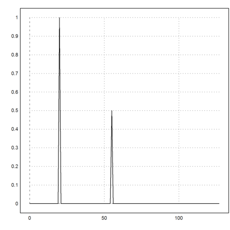
The following signal is made of the frequencies 20 and 55.
>t=0:Pi/128:2*Pi-Pi/128; s=2*cos(20*t)+cos(55*t);
We can see these frequencies with a Fourier transformation.
>f=abs(ifft(s)); plot2d(0:127,f[1:128]):
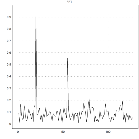
Adding randomly distributed noise does still shows the frequencies clearly.
>s=s+normal(size(s)); f=abs(ifft(s)); plot2d(0:127,f[1:128],title="FFT"):
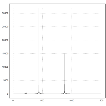
Euler can generate sound using its matrix language. The sound can be saved in WAV format and played back by the system.
At first we create 2 seconds of sound parameters.
>t=soundsec(2);
Then we generate the sound.
>s=sin(440*t)+sin(220*t)/2+sin(880*t)/2;
We can easily make a Fourier analysis of it.
>analyzesound(s):
If you have speakers on, you can hear the sound file.
>playwave(s);
Now we add a lot of noise and listen to it.
>sa=s+normal(size(s)); playwave(sa);
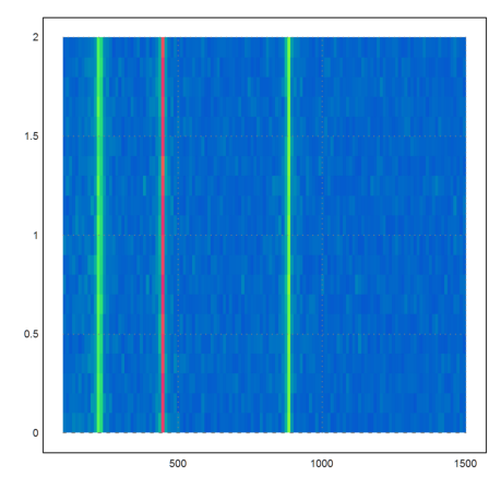
We can also make a picture of the sound frequencies versus the length of the sound.
>mapsound(sa):
The Fourier transformation has a very interesting property. The folding of two sequences is defined as
![]()
E.g., if we fold a sequence a with b=[1/2,1/2], we take the average of two neighboring elements, with a[0]=a[n], a[-1]=a[n-1] etc. This can be computed by a simple multiplication of the Fourier transformation.
>a=1:8; b=[0.5,0.5,0,0,0,0,0,0]; real(ifft(fft(a)*fft(b)))
[4.5, 1.5, 2.5, 3.5, 4.5, 5.5, 6.5, 7.5]
There is a function for this in EMT.
>fftfold(a,[0.5,0.5])
[4.5, 1.5, 2.5, 3.5, 4.5, 5.5, 6.5, 7.5]
There is also fold(), which uses a loop to compute the fold, but does not go modulo n. Consequently, the resulting vector is shorter.
>fold(a,[0.5,0.5])
[1.5, 2.5, 3.5, 4.5, 5.5, 6.5, 7.5]
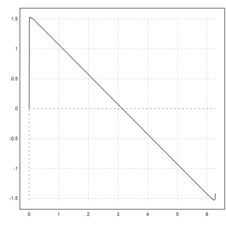
Finally, we are going to demonstrate Gibbs phenomenon. Summing up sin(nt)/n for odd n approaches a triangle wave form but with an error at 0 and pi.
>t=linspace(0,pi,500)';
To compute the sum sin(k*t)/k of k=1,...,100, we use the matrix language of Euler.
>s=sum(sin(t*(1:100))/(1:100))*2;
The plot shows that the Fourier sum converges to pi-x.
>plot2d(t',s'); plot2d("pi-x",color=3,add=1):
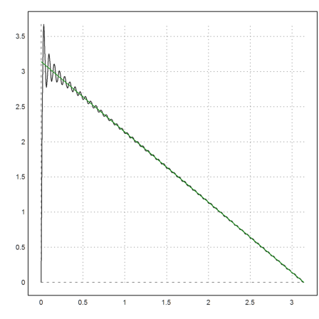
But there is an overshoot close to 0, which is called Gibbs phenomenon. Let us measure this overshoot for a very large n.
>t=linspace(0,pi,5000)'; max(sum(sin(t*(1:1000))/(1:1000))'*2-(pi-t'))
0.5622809267763276
Using a Riemann sum, one can see that the limit of this value for n to infinity is the following.
>integrate("sinc(x)",0,pi)*2-pi
0.5622814503751381
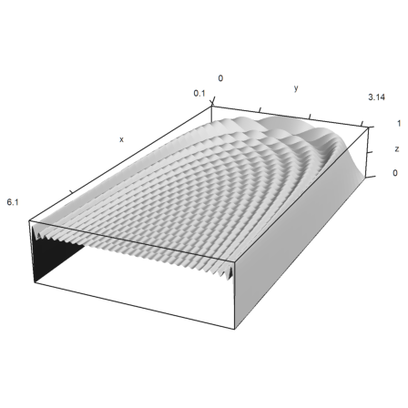
Let us plot some the truncated series for n=1,3,...,61 using a 3D plot.
>n=1:2:61; ...
 t=linspace(0,pi,500)'; ...
 S=cumsum(sin(t*n)/n); ...
 plot3d(n/10,t,S,hue=1,zoom=5):