Euler has some useful functions for geometry. Most functions are implemented in numerical and also in symbolic form. You have to load the geometry file before using the functions.
>load geometry
Numerical and symbolic geometry.
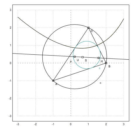
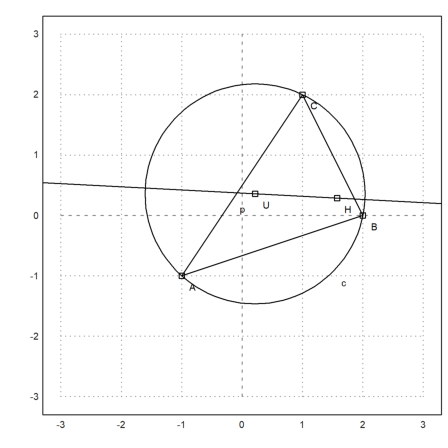
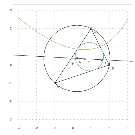
For a demonstration, we compute and plot the Euler line in a triangle. The following construction has been done with C.a.R. and shows the result we wish to achieve.
First, we define the corners of the triangle in Euler. We use a definition, which is visible in symbolic expressions.
>A::=[-1,-1]; B::=[2,0]; C::=[1,2];
To plot geometric objects, we setup a plot area, and add the points to it. All plots of geometric objects are added to the current plot.
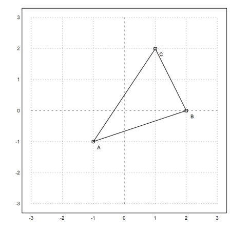
>setPlotRange(3); plotPoint(A,"A"); plotPoint(B,"B"); plotPoint(C,"C");
We can also add the sides of the triangle.
>plotSegment(A,B,""); plotSegment(B,C,""); plotSegment(C,A,""):
Here is the area of the triangle, using the determinant formula. Of course, we have to take the absolute value of this result.
>&areaTriangle(A,B,C)
                                   7
                                 - -
                                   2
We can compute the coefficients of the side c.
>c &= lineThrough(A,B)
[- 1, 3, - 2]
And also get a formula for this line.
>&getLineEquation(c,x,y)
3 y - x = - 2
For the Hesse form, we need to specify a point, such that the point is on the positive side of the Hesseform. Inserting the point yields the positive distance to the line.
>&getHesseForm(c,x,y,C), &at(%,[x=C[1],y=C[2]])
                             3 y - x + 2
                             -----------
                              sqrt(10)


                                  7
                               --------
                               sqrt(10)
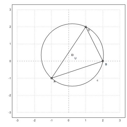
Now we compute the circumcircle of ABC.
>Cu &= circleThrough(A,B,C); &getCircleEquation(Cu,x,y)
                          5  2        3  2   325
                     (y - --)  + (x - --)  = ---
                          14          14     98
>U &= getCircleCenter(Cu)
                                3   5
                               [--, --]
                                14  14
Plot the circle and its center. Cu and U are symbolic. We evaluate these expressions for Euler.
>plotCircle(Cu()); plotPoint(U(),"U"):
We can compute the intersection of the heights in ABC (the orthocenter) numerically with the following command.
>H &= lineIntersection(perpendicular(A,lineThrough(C,B)),...
   perpendicular(B,lineThrough(A,C)))
                                11  2
                               [--, -]
                                7   7
Now we can compute the Euler line of the triangle.
>el &= lineThrough(H,getCircleCenter(Cu)); &getLineEquation(el,x,y)
                            19 y   x      1
                          - ---- - -- = - -
                             14    14     2
Add it to our plot.
>plotPoint(H(),"H"); plotLine(el()):
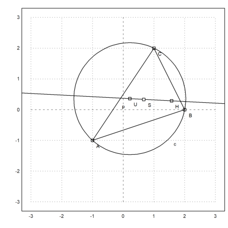
The gravitational center should be on this line.
>S &= (A+B+C)/3; &getLineEquation(el,x,y) with [x=S[1],y=S[2]]
                                1     1
                              - - = - -
                                2     2
>plotPoint(S(),"S"):
The theory tells us SH=2*SU. We need to simplify with radcan to achieve this.
>&distance(S,H)/distance(S,U)|radcan
2
The functions include functions for angles too.
>&computeAngle(A,C,B), deg(%())
                                    4
                        acos(----------------)
                             sqrt(5) sqrt(13)

60.2551187031
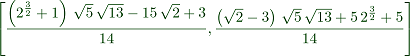
The equation for the center of the incircle is not very nice.
>Is &= lineIntersection(angleBisector(A,C,B),angleBisector(C,B,A))|radcan
           3/2
         (2    + 1) sqrt(5) sqrt(13) - 15 sqrt(2) + 3
        [--------------------------------------------,
                              14
                                                              3/2
                          (sqrt(2) - 3) sqrt(5) sqrt(13) + 5 2    + 5
                          -------------------------------------------]
                                              14
In Latex, this prints as
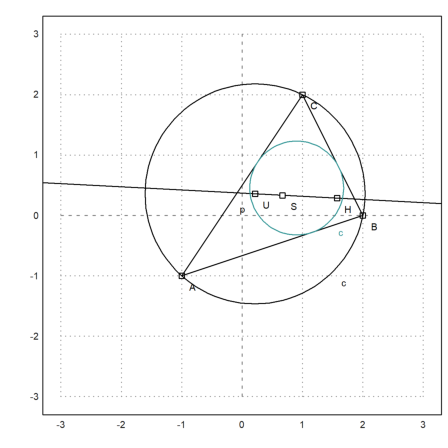
Let us compute also the expression for the radius of the inscribed circle.
>ri &= distance(Is,projectToLine(Is,lineThrough(A,B)))|ratsimp
        sqrt((- 41 sqrt(2) - 31) sqrt(5) sqrt(13) + 115 sqrt(2) + 614)
        --------------------------------------------------------------
                                  7 sqrt(2)
>Ci &= circleWithCenter(Is,ri);
Let us add this to the plot.
>color(5); plotCircle(Ci()):
Next, we find an equation for the points with equal distance from C to AB.
>eq &= getHesseForm(lineThrough(A,B),x,y,C)-distance([x,y],C)
               3 y - x + 2               2          2
               ----------- - sqrt((2 - y)  + (1 - x) )
                sqrt(10)
Using Euler's level plot, we can add this to plot.
>plot2d(eq,level=0,add=1,contourcolor=6):
This should be some function, but the default solver of Maxima can find the solution only, if we square the equation. Consequently, we get a fake solution.
>seq &= solve(getHesseForm(lineThrough(A,B),x,y,C)^2-distance([x,y],C)^2,y)
        [y = - 3 x - sqrt(70) sqrt(9 - 2 x) + 26,
                              y = - 3 x + sqrt(70) sqrt(9 - 2 x) + 26]
The first solution is
![]()
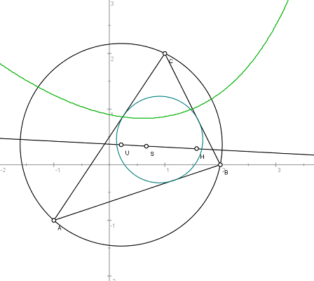
Adding the first solution to the plot show, that it is indeed the path we are looking for. The theory tells us that it is a rotated parabola.
>plot2d(&rhs(seq[1]),add=1):