Often in mathematics, we encounter linear problems with a large number of coefficients and equations, but only a few non-zero coefficients. For this, Euler Math Toolbox has a special matrix type with a compressed format.
The following reference contains all relevant functions.
In this tutorial, we demonstrate how to use the cpx functions of Euler for compressed large matrices.
First, we generate a matrix with a band structure.
>n=5; A=id(n)*2+diag(n,n,-1,1)+diag(n,n,1,1); fracprint(A);
        2         1         0         0         0
        1         2         1         0         0
        0         1         2         1         0
        0         0         1         2         1
        0         0         0         1         2
This matrix can be compressed into a data structure containing only a list of the elements different from 0.
>R=cpx(A)
Compressed 5x5 matrix
    1     1                    2
    1     2                    1
    2     1                    1
    2     2                    2
    2     3                    1
    3     2                    1
    3     3                    2
    3     4                    1
    4     3                    1
    4     4                    2
    4     5                    1
    5     4                    1
    5     5                    2
The compression really pays in the case of huge matrices.
We could build the matrix like the matrix above as a full matrix and compress later. But there are methods to build such a matrix as a compressed matrix.
>n=1000; R=cpxzeros(n,n);  ...
   R=cpxsetdiag(R,0,2); R=cpxsetdiag(R,1,1); R=cpxsetdiag(R,-1,1);
Multiplication of two such matrices is much faster than multiplication of the orginal matrices.
For a 1000x1000 matrix like the one above, we would need one billion (1000^3) multiplications. The compressed format needs only a few thousand.
>cpxmult(R,R);
Using iterative methods, we can solve such large systems. For a demonstration, we call the cpxfit function, which uses the conjugate gradient method for R'Rx=R'b. It works even for 1000 equations of 1000 unknowns.
We use for b the sum of the rows of A. The correct solution would be x[j]=1 for all j.
>b=cpxsum(R); ...
 x=cpxfit(R,b); ...
 totalmax(cpxmult(R,x)-b)
2.27965202271e-010
Here is another example with a random matrix. We first define an empty 1000x1000 matrix.
>H=cpxzeros(1000,1000);
Then we 10000 create random indices, which we want to set to a random number later.
>ind=intrandom(10000,2,1000);
The indices are now a 2x10000 matrix of the form
i[1],j[1]
i[2],j[2]
...
Now set those indices in H to a random number. For this we use cpxset, which needs a matrix with rows
i,j,x
...
and sets R[i,j] to x.
>H=cpxset(H,ind|normal(rows(ind),1));
Finally, we set the diagonal of H to a large number to avoid non-regular matrices.
>H=cpxsetdiag(H,0,20);
Define b equal to the sum of the rows in H.
>b=cpxsum(H);
Solve the system. The solution should be all ones, so the difference should be 0.
>totalmax(cpxfit(H,b)-1)
0
The function cpxget extracts all elements in the form
i,j,x
We extract the elements with row index 1.
>r=cpxget(H); r1=nonzeros((r[,1]==1)'); r[r1]
            1             1            20
            1            73     -0.657814
            1           111      -1.55385
            1           187    -0.0660178
            1           233       1.05364
            1           493      0.312246
            1           515      0.927542
            1           562      0.495431
            1           636      0.484003
            1           646      -1.36699
            1           714    -0.0810937
            1           719      0.629548
            1           756      -1.68859
Here is an example, where we compute the resistance of a rectangular grid of size 50x50 from corner to corner. The grid has 2500 grid points, which will be the number of variables of the linear systems.
Each connection has a resistance of 1. The flow of current between two points is the difference in voltage divided by the resistance (1 in this case). The sum of the flows must be 0. So the voltage in each point must be the average of the voltages of the points connected to this point.
>n=50;
The function rectangleIncidenceX returns the incidence matrix of the grid. It is of size n^2 times n^2 and has 1 in R[i,j], if point i is connected with point j.
>R=rectangleIncidenceX(n,n);
We compute the numbers of edges going from each point, and divide the rows by that number.
>c=cpxsum(R); R=cpxmultrows(1/c,R);
Now we set the diagonal to -1. The system R.x=0 is now satisfied by all voltages x, such that each point is the average of all neighboring points.
>R=cpxsetdiag(R,0,-1);
Now we add the condition that the first point has voltage 1, and the last has voltage 0.
>R=cpxsetrow(R,1,0); R=cpxset(R,[1,1,1]); ...
 R=cpxsetrow(R,n^2,0); R=cpxset(R,[n^2,n^2,1]); ...
 b=zeros(n^2,1); b[1]=1;
We solve for R.x=b, using the conjugate gradient method with thin matrices for
![]()
It takes a few seconds for this large matrix.
>x=cpxfit(R,b);
Now plot the lines of equal voltage.
>plot2d(redim(x,n,n),a=1,b=50,c=1,d=50,hue=1,>contour,>spectral):
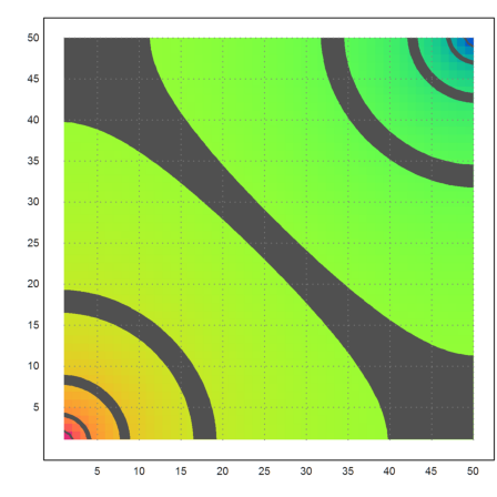
In this case the total resistance is 1 over the current flow out of the corner point. Flowing along each connection is a current equal to the differences of voltages, since the resistance is 1. Note that the connected points have numbers 2 and n+1.
>1/(2*x[1]-x[2]-x[n+1])
5.05836762787