In this demo, I like to show you the range of nice graphics Euler can produce.
The easiest way to obtain a plot in Euler is an expression. The default range is from -2 to 2. The y-range is automatic.
For the demo, we change the range from -2 to 1.
>plot2d("x^3+x^2-x",-2,1):
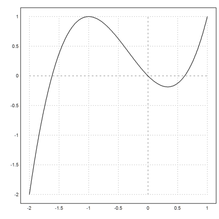
Note the colon ":" after the plot, which inserts the plot into the notebook.
For the following plot, we change the aspect ratio of the plot. To plot more than one functions, the easiest way is to use an array of expressions.
>aspect(2); plot2d(["sin(x)","cos(x)"],0,2pi,-1.2,1.2):
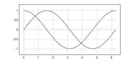
If you have changed the aspect but do not want to keep it permanently reset the aspect() with the following command.
>aspect();
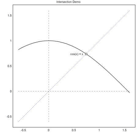
Another way to set the range is with a radius r. The center is (0,0) by default, but we can chose any other center. (An alternative is to set a,b,c,d parameters for the plot window [a,b]x[c,d]).
For the demo, we plot two functions in different colors and styles into one plot. Moreover, we change the grid type using less grid lines.
>plot2d(["cos(x)","x"],r=1.1,cx=0.5,cy=0.5, ...
   color=[black,blue],style=["-","."], ...
   grid=1);
If you do not see this plot in your window layout, press the tabulator key.
We add the intersection point with a label (at position "cl" for center left), and insert the result into the notebook. We also add a title to the plot.
>x0=solve("cos(x)-x",1);  ...
   plot2d(x0,x0,>points,>add,title="Intersection Demo");  ...
   label("cos(x) = x",x0,x0,pos="cl",offset=20):
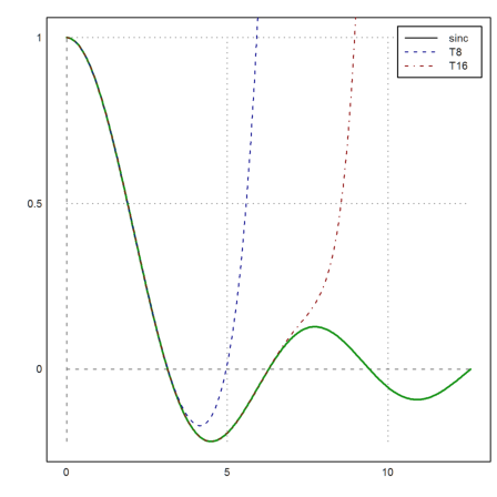
In the following demo, we plot the sinc(x) function and its 8-th and 16-th Taylor expansion. We compute this expansion using Maxima via symbolic expressions.
>&taylor(sin(x)/x,x,0,4)
                              4     2
                             x     x
                             --- - -- + 1
                             120   6
This plot is done in the following multi-line command with three calls to plot2d(). The second and the third have the >add flag set, which makes the plots use the previous ranges.
We add a label box explaining the functions.
>plot2d("sinc(x)",0,4pi,color=green,thickness=2); ...
   plot2d(&taylor(sin(x)/x,x,0,8),>add,color=blue,style="--"); ...
   plot2d(&taylor(sin(x)/x,x,0,16),>add,color=red,style="-.-"); ...
   labelbox(["sinc","T8","T16"],styles=["-","--","-.-"], ...
     colors=[black,blue,red]):
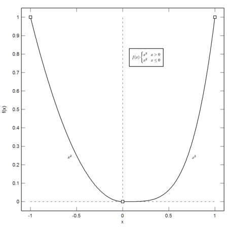
Of course, functions can also be used.
>function map f(x) ...
 if x>0 then return x^4
 else return x^2
 endif
 endfunction
The "map" parameter helps to use the function for vectors. For the plot, it would not be necessary. But to demonstrate that vectorization is useful, we add some key points to the plot at x=-1, x=0 and x=1.
In the following plot, we also enter some LaTeX code. We use it for two labels and a text box. Of course, you will only be able to use LaTeX if you have LaTeX installed properly.
>plot2d("f",-1,1,xl="x",yl="f(x)",grid=6);  ...
 plot2d([-1,0,1],f([-1,0,1]),>points,>add); ...
 label(latex("x^3"),0.72,f(0.72)); ...
 label(latex("x^2"),-0.52,f(-0.52),pos="ll"); ...
 textbox( ...
   latex("f(x) \begin{cases} x^3 & x>0 \\ x^2 & x \le 0\end{cases}"), ...
   x=0.7,y=0.2):
You can change the default grid style globally. We do that in the next plot.
Moreover, we use Unicode strings in the following plot. Unicode strings can be used in all plot texts. This may often be an alternative to LaTeX.
>gridstyle(st1="->",color=blue,textcolor=blue); ...
plot2d("x^3+x-x^2",0,1,grid=3,style="--",<frame,>vertical); ...
labelbox(u"x³ + x - x²","--",x=0.5,y=0.2,style="t"):
Revert to the default styles and colors with reset().
>reset;
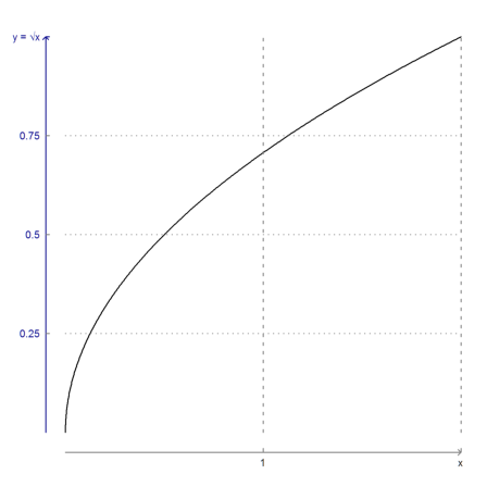
For even more control, each axis can be plotted separately.
In the example, we plot the y axis twice, once for the axis and the label, and once for the ticks. For demonstration, we use a blue color. Moreover, we position the axes to the left and below the plot. For this, the first parameter of yaxis() and xaxis() determines the exact position of the axis.
>plot2d("sqrt(x)",0,1,<frame,grid=0); ...
yaxis(-0.05,1,u"y = √x",style="->",color=blue,textcolor=blue); ...
yaxis(-0.05,0.25:0.25:0.75,>grid,<axis,>left,textcolor=blue); ...
xaxis(-0.05,[0.5,1],["1","x"],style="->",>grid,gridstyle="--"):
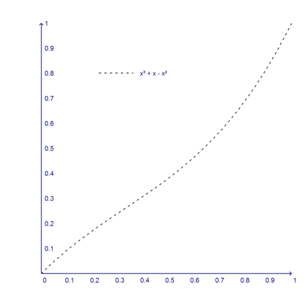
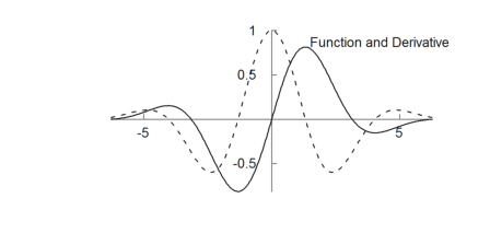
Often, you will need an EMT plot for a scientific paper or a book. Then the label size must of the plot should match the text size.
With setfont(), a new font can be chosen. You need the font size and the output height. What parameters actually look best might need a bit of experimenting.
>setfont(10pt,12cm); aspect(2); expr&=sin(x)*exp(-x^2/10); ...
 plot2d([expr,&diff(expr,x)],-2pi,2pi,style=["-","--"],grid=7,<frame); ...
 textbox("Function and Derivative",color=transparent):
If you need b/w plots and don't want to set each individual plot, you can disable colors in the Options menu. Then the notebook colors will also be mapped to shades of gray.
We need to reset() to the defaults to continue with this introduction.
>reset();
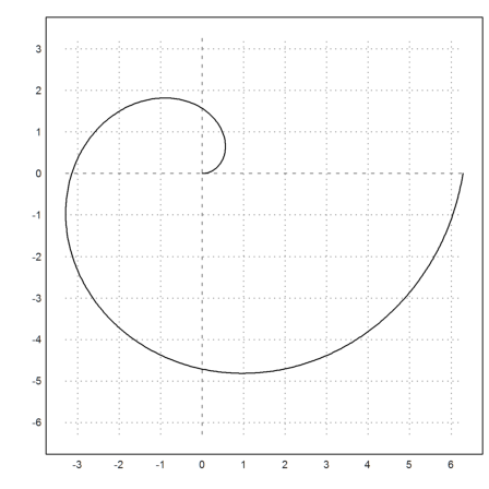
The easy way to plot parametric curves are two expressions.
In the example, we plot the spiral of Archimedes. To keep the plot square we set the >square parameter. Then the x-range is automatic, but the y-range is centered, so that the plot range is a square in the plane.
>plot2d("x*cos(x)","x*sin(x)",xmin=0,xmax=2pi,>square):
The main point of the matrix language is that it allows to generate tables of functions easily.
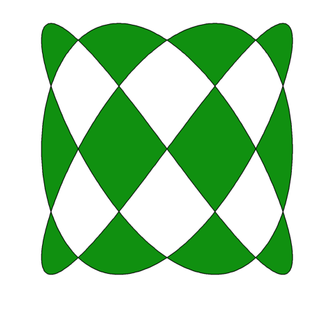
>t=linspace(0,2pi,1000); x=cos(3*t); y=sin(4*t);
We now have vectors x and y of values. plot2d() can plot these values as a curve connecting the points. The plot can be filled. In this case this yields a nice result due to the winding rule, which is used for the fill.
>plot2d(x,y,<grid,<frame,>filled):
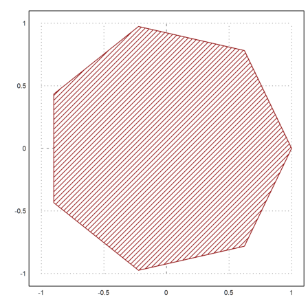
Another example is a septagon, which we create with 7 points on the unit circle.
>t=linspace(0,2pi,7);  ...
  plot2d(cos(t),sin(t),r=1,>filled,style="/",fillcolor=red):
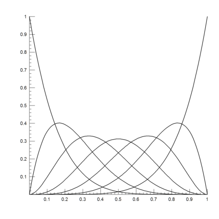
We can also plot one row of x-values with many rows of y values. To generate such a matrix, we use the matrix language of Euler.
>x=0:0.01:1; n=(0:6)'; y=bin(6,n)*x^n*(1-x)^(6-n);
We now have
![]()
These are tables of the Bernstein polynomials in [0,1].
>plot2d(x,y,grid=8,<frame):
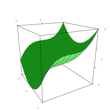
We need a 3D plot to visualize a function of two variables.
Euler draws such functions using a sorting algorithm to hide parts in the background. The projection is a central projection. The view angle and height can be changed. The default is from the positive x-y quadrant, but angle=0° looks from into the direction of the y-axis.
>plot3d("x^2+y^3",r=1,angle=60°,height=20°,zoom=2.5):
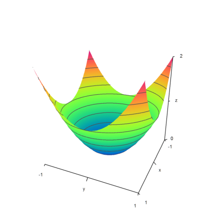
For the plot, Euler adds grid lines. Instead it is possible to use level lines and a one-color hue or a spectral colored hue.
>plot3d("x^2+y^2",levels=-2:0.2:2,>spectral,n=100,frame=3,zoom=2.2):
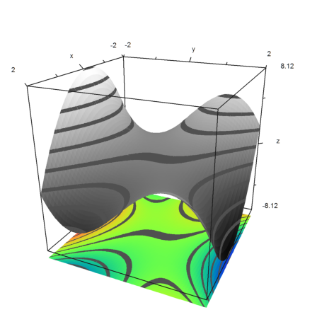
The following plot uses level lines, which indicate the area, where the function is between two limits. The width of the limits can be set by dl. We use the default value.
We add a contour plane below the plot showing the values in spectral colors.
>plot3d("x^2*y-y^3-x",r=2,>contour,>cp,cpcolor=spectral):
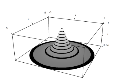
A polar plot is also available.
The parameter "fscale" scales the function with an own scale. Otherwise the function is scaled to fit into a cube.
>aspect(1.5);  ...
   plot3d("1/(x^2+y^2+1)",r=5,>polar, ...
     fscale=2,>hue,n=100,zoom=4,>contour,color=gray):
Euler can plot parameterized surfaces too, when the parameters are the x-, y-, and z-values of an image of a rectangular grid in the space.
For the following demo, we setup u- and v- parameters, and generate space coordinates from these.
>u=linspace(-1,1,10); v=linspace(0,2*pi,50)'; ...
  X=(3+u*cos(v/2))*cos(v); Y=(3+u*cos(v/2))*sin(v); Z=u*sin(v/2); ...
  plot3d(X,Y,Z,>anaglyph,<frame,>wire,scale=2.3):
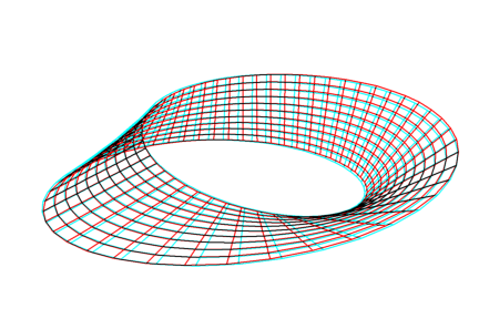
This plot is an anaglyph plot. You need to use red/cyan glasses to experience the nice 3D effect.
Do not forget to reset the aspect.
>aspect(); ...
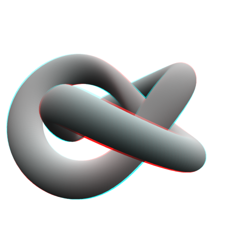
Here is a more complicated example, which is majestic with red/cyan glasses.
>u:=linspace(-pi,pi,160); v:=linspace(-pi,pi,400)'; ...
   x:=(4*(1+.25*sin(3*v))+cos(u))*cos(2*v); ...
   y:=(4*(1+.25*sin(3*v))+cos(u))*sin(2*v);  ...
   z=sin(u)+2*cos(3*v); ...
 plot3d(x,y,z,frame=0,scale=1.5,hue=1,light=[1,0,-1],zoom=2.8,>anaglyph):
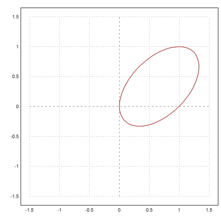
Euler can mark the level lines
![]()
of any function.
>plot2d("x^2+y^2-x*y-x",r=1.5,level=0,contourcolor=red):
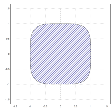
It is also possible to fill the set
![]()
with a level range.
>plot2d("x^4+y^4",r=1.5,level=[0;1],color=blue,style="/"):
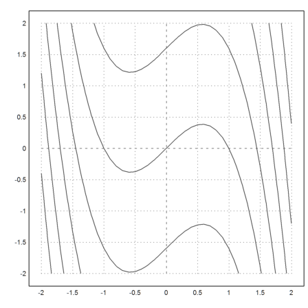
>plot2d("x^3+y-x",r=2,>contour,level="thin"):
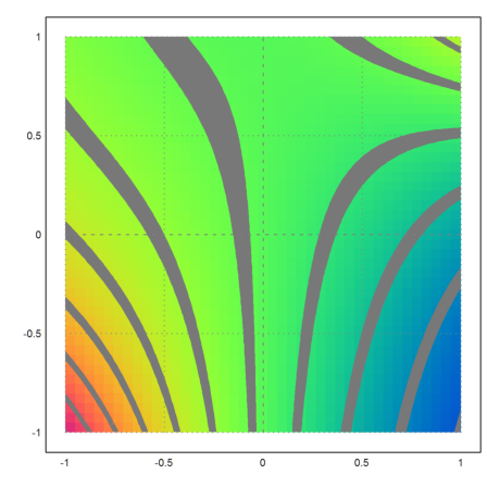
There is also an automatic style showing some ranges of level lines. You can add a background shading.
>plot2d("exp(x*y)-x",>contour,>hue,contourcolor=gray,>spectral):
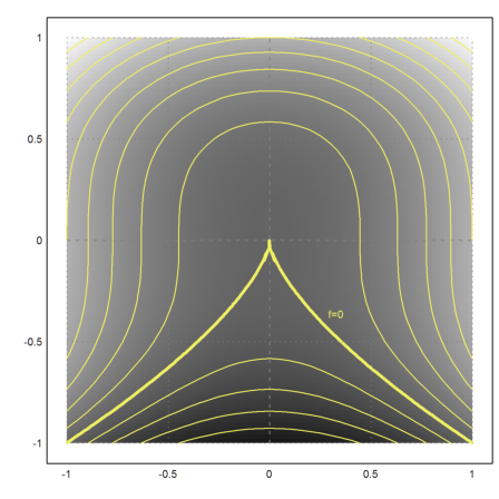
In the following example, we emphasize one level line. To do this, we add the less important lines later.
>plot2d("x^2+y^3",level=0, ...
     contourwidth=3,contourcolor=yellow,color=black,>hue,n=100); ...
   plot2d("x^2+y^3",level=-2:0.2:2,contourcolor=yellow,>add); ...
   label("f=0",0.25,-0.3,color=yellow):
Here is another style of contour lines.
>plot2d("x^2+x*y",>contour,n=100):
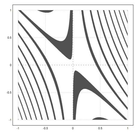
It is also possible to mark a region
![]()
This is done by adding a level with two rows.
>plot2d("(x^2+y^2-1)^3-x^2*y^3",r=1.3, ...
   style="#",color=red,<outline, ...
   level=[-2;0],n=100):
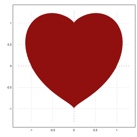
We wish to turn this around the y-axis. Here is the expression, which defines the heart.
>expr &= (x^2+y^2-1)^3-x^2*y^3
                          2    2     3    2  3
                        (y  + x  - 1)  - x  y
Now we set
![]()
>function fr(r,a) &= expr with [x=r*cos(a),y=r*sin(a)] | trigreduce
                                                         5
             2     3   (sin(5 a) - sin(3 a) - 2 sin(a)) r
           (r  - 1)  + -----------------------------------
                                       16
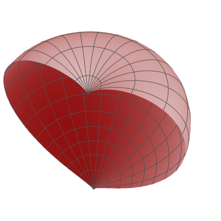
This allows to define a numerical function, which solves for r, if a is given. With that function we can plot the turned heart as a parametric surface.
>function map f(a) := bisect("fr",0,2;a); ...
 t=linspace(-pi/2,pi/2,100); r=f(t); ...
 s=linspace(pi,2pi,100)'; ...
 plot3d(r*cos(t)*sin(s),r*cos(t)*cos(s),r*sin(t), ...
   >hue,<frame,color=red,zoom=4,amb=0,max=0.7,grid=12,height=50°):
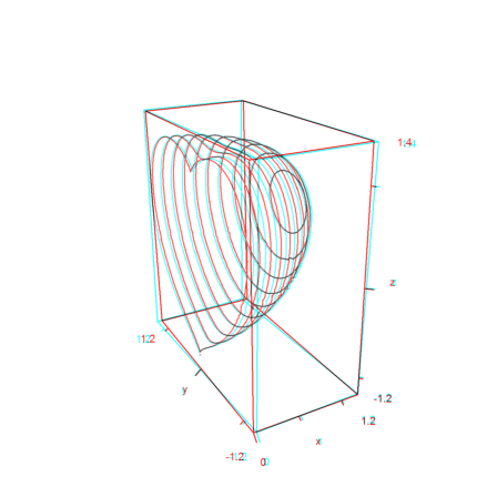
There are also implicit 3D plot. Euler generates cuts through the objects.
The following is a 3D plot of the figure above rotated around the z-axis. We define the function, which describes the object.
>function f(x,y,z)  ...
 r=x^2+y^2;
 return (r+z^2-1)^3-r*z^3;
 endfunction
The plot is an anaglyph plot. You need red/cyan glasses to view it properly.
>plot3d("f(x,y,z)", ...
   xmin=0,xmax=1.2,ymin=-1.2,ymax=1.2,zmin=-1.2,zmax=1.4, ...
   implicit=1,angle=-30°,zoom=2.5,n=[10,60,60],>anaglyph):
Euler has many statistical plots. See
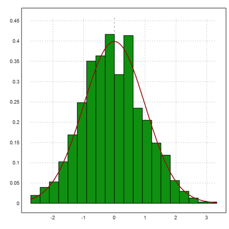
For a simple distribution, we can use >distribution in plot2d.
>plot2d(normal(1,1000),>distribution); ...
   plot2d("qnormal(x)",color=red,thickness=2,>add):
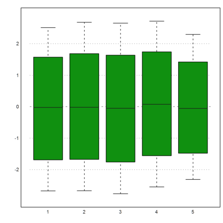
There are also many special plots for statistics.
>M=normal(5,1000); boxplot(quartiles(M)):
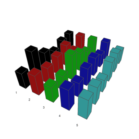
The following are 5 runs of 100 dice throws. We count the numbers of 1s to 6s in each throw.
>Z=intrandom(5,100,6); v=zeros(5,6); ...
   loop 1 to 5; v[#]=getmultiplicities(1:6,Z[#]); end; ...
   columnsplot3d(v',scols=1:5,ccols=[1:5]):