by R. Grothmann
I have been inspired to look at ugly distributions by the book "Black Swans" by N.N.Talib. He claims that such distributions are more real life than the standard "bell curve". A black swan is a rare, but important event, which is essentially unpredictable. Ugly distributions are distributions, which can produce black swans.
Black Swan Theory on Wikipedia
Mathematically, we are talking about the Cauchy distribution, or distributions of Pareto type.
This notebook also contains a study of the distribution of the deltas of the DAX (German stock index).
To compare good and bad distributions, let us start with the Gauß distribution, which is of course a good distribution. What is the mean distance, a random walk will travel? How would a random walk "look like"?
>&assume(n>0);
First, we investigate a 0-1-normal distributed random walk. The expected absolute distance of n steps of the walk can be computed by integrating |x| with respect to this distribution.
![]()
Due to symmetry, we can use the following integral.
>&2*integrate(sqrt(n)/sqrt(2*pi)*exp(-n*x^2/2)*x,x,0,inf)
                               sqrt(2)
                           ----------------
                           sqrt(pi) sqrt(n)
Let us generate a Monte-Carlo simulation of random walks with 0-1-normal distributed steps.
With the following command, we do 1000 random walks of length 1000, and print the mean value of the absolute distance, as well as the standard deviation of it.
>n:=1000; S:=abs(sum(normal(1000,n))'); mean(S), dev(S)
25.4323731799
18.9065448062
The expected distance from 0 is
>sqrt(2/(pi*n))*n
25.2313252202
Note that the deviation of the traveling distance is quite large. This means, that it is difficult to predict the distance, even in this "normal" case.
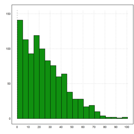
Here is the simulated distribution of the absolute walking distance of our 1000 random walks of length 1000.
>{x,y}=histo(S,20); plot2d(x,y,bar=1):
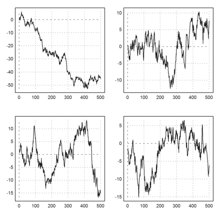
For an optical impression, the following plot shows four such walks.
>figure(2,2); loop 1 to 4; figure(#); plot2d(cumsum(normal(1,500))); end; ...
 insimg; figure(0);
Due to the strong law of large numbers, the same behavior is to be expected by all random walks with variance 1 in each step.
Here is a {-1,1}-walk, which takes steps -1 or 1 with probability 1/2.
>n:=1000; S:=abs(sum(intrandom(n,n,2)*2-3)'); mean(S), dev(S)
25.602
19.7746462075
>{x,y}=histo(S,20); plot2d(x,y,bar=1):
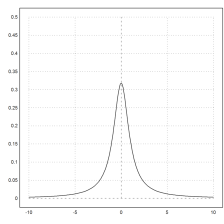
Now we consider some ugly distributions for the steps. The following distribution is called the Cauchy distribution.
![]()
This distribution has neither an expected value, nor a variance, just like the distributions in Taleb's book.
>expr &= 1/(pi*(1+x^2)); plot2d(expr,a=-10,b=10,c=0,d=0.5):
The distribution is a probabilistic random distribution.
>&integrate(expr,x,-inf,inf)
1
The probability of a larger value than a behaves like pi/a. This does not go toward 0 so rapidly.
To see this behavior, we develop the cumulative distribution P(x<=a) near infinity;.
>&assume(a>0); &taylor(integrate(@expr,x,a,inf),a,inf,2)
                                  1
                                 ----
                                 pi a
To simulate this distribution, we solve P(x<=a)=y for a.
>&solve(integrate(expr,x,-inf,a)=y,a)
[a = - cot(pi y)]
Then, we choose y uniformly in [0,1], and return the corresponding a.
>function prand(n,m) := -1/tan(pi*random(n,m))
If we run a simulation of this distribution, we often get large values. These are the black swans of Teleb's book.
>s:=prand(1,1000); plot2d(s,distribution=20):
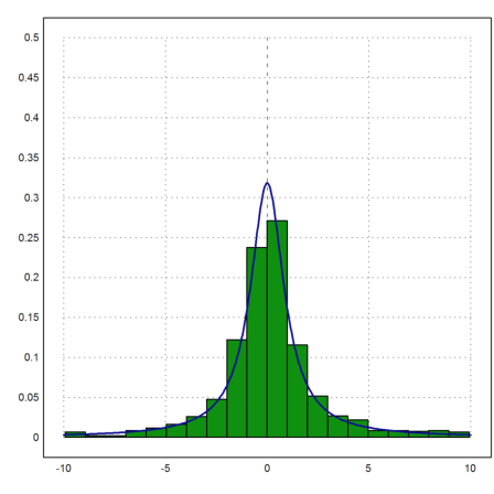
However, if we truncate the large values (plot only the values close to 0), we can see the Cauchy distribution.
>s:=prand(1,1000); s=s[nonzeros(abs(s)<10)]; ...
 plot2d(s,a=-10,b=10,c=0,d=0.5,distribution=20); ...
 plot2d(expr,add=1,thickness=2,color=blue):
How about a random walk with this distribution?
>n:=1000;
Most probably, we get a very large walking distance, and an even larger deviation. We cannot predict, how large the sum of n such random variables is. This is due to the large excessive values of the distribution.
>S:=abs(sum(prand(1000,n))'); mean(S), dev(S)
4395.69627879
19169.1503693
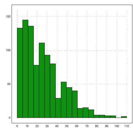
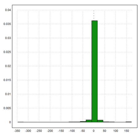
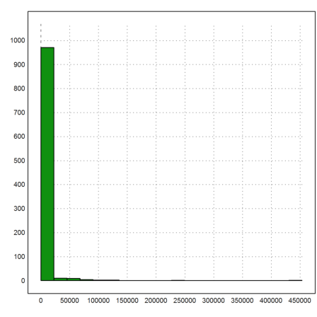
The plot of the absolute walking distances over all simulated walks show this clearly.
>plot2d(S,histogram=20):
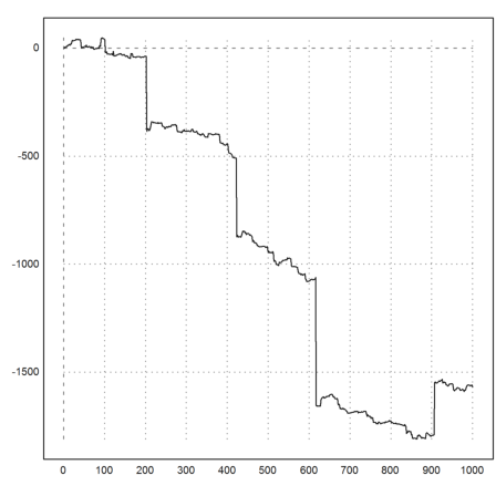
Here is a single random walk. It makes huge steps sometimes. In some periods, it looks very ordinary. This behavior simulates black swans, which are rare, decisive, unexpected events.
>plot2d(cumsum(prand(1,1000))):
Let us take a not so bad distribution. The following distribution has an expected value (0), but no variance.
![]()
It is of the same type as the so called Pareto distributions.
>&1/(2*integrate(1/(1+x^3),x,0,inf))
                                  3/2
                                 3
                                 ----
                                 4 pi
We put the scaled density function into an expression, and test, if it is really a probabilistic distribution.
>expr1 &= 3*sqrt(3)/(4*%pi*(1+abs(x)^3));  ...
 & 2*integrate(expr1,x,0,inf)
1
We can compute P(x>=a) with Maxima, but the expression is not so nice.
>&assume(a>0,a^2-a+1>0);  ...
 function distr(a) &=1-integrate(expr1,x,a,inf)
                                         2 sqrt(3) a - sqrt(3)
                       2            atan(---------------------)
             3/2  log(a  - a + 1)                  3
       1 - (3    (--------------- - ---------------------------
                         6                    sqrt(3)
                                       log(a + 1)      pi
                                     - ---------- + ---------))/(4 pi)
                                           3        2 sqrt(3)
It behaves like 1/a^2 as already expected from the density function. First a numerical test.
>plot2d(&(1-distr(x))*x^2,0,100):
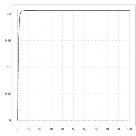
Here is a symbolic proof of this.
>&limit((1-distr(a))*a^2,a,inf), %()
                                  3/2
                                 3
                                 ----
                                 8 pi

0.206748335783
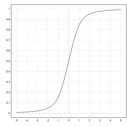
Let us define this cumulative distribution in Euler.
>function map distr(a) ...
 if a>0 then return &:distr(a)
 else return 1-(&:distr(-a))
 endif
 endfunction
>plot2d("distr",-5,5):
We define the inverse to this cumulative distribution. We use a mixture of the bisection and the secant method.
>function map invdistr(b) ...
 if b>distr(1000) then return 1000;
 else if b<distr(-1000) then return -1000;
 else
   x=bisect("distr",-1000,1000,y=b,eps=1);
   return secantin("distr",x-1,x+1,y=b);
 endif;
 endfunction
>invdistr(0.2), distr(%)
-0.808667971095
0.2
Then we can define a random variable for this.
>function p1rand(n,m) := invdistr(random(n,m))
This is okay for a small number of random values.
>plot2d(p1rand(1,1000),>distribution):
We can improve the generation of random number for this distribution with the restriction method. If g and f are density functions of two random variables and g<cf for some constant then we can generate samples for g by accepting a sample value x from f if
![]()
where a(x) is uniformly distributed in [0,1]. Here is a function with c=1 and
![]()
>function p1randr(n,m) ...
 k=n*m;
 v=[];
 repeat
   w=prand(1,2*k);
   f=random(1,2*k);
   i=nonzeros(2*f/(1+w^2)<1/(1+abs(w)^3));
   v=v|w[i];
   until length(v)>k;
 end;
 return redim(v[1:k],n,m);
 endfunction
As you see, we first generate a vector of length n*m and form a matrix from this vector at the end.
We can now generate much larger samples.
>n:=1000; S:=abs(sum(p1randr(1000,n))'); mean(S), dev(S)
54.1183829352
55.252107923
Just to make sure, we compare the two generators with an quantile plot.
>plot2d(sort(p1randr(1,1000)),sort(p1rand(1,1000)),r=5,>points):
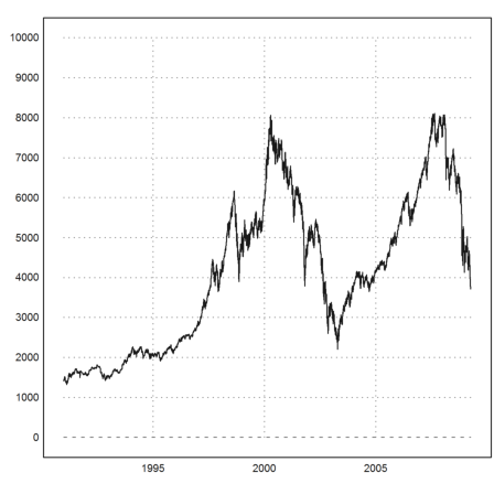
For a real life example, we study the development of the German stock index DAX. I have put the data, collected over the past 18 years on a daily basis, into a data file. The time is backwards, so we need to flip it.
>dax:=flipx(readmatrix("kurs.dat")');
The 4th column in the file is the rate. The first three columns contain the date.
>rate:=dax[4]; date:=dax[1]+(dax[2]+dax[3]/31)/12; ...
 plot2d(date,rate,a=date[1],b=date[-1],c=0,d=10000):
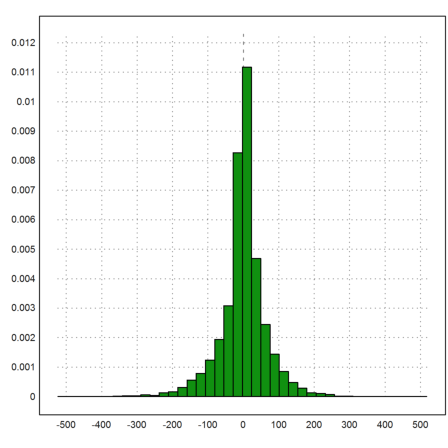
We want to study the deltas
![]()
and plot the distribution of these deltas.
>n:=cols(rate); delta:=differences(rate);
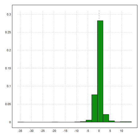
Now we can plot the distribution of the deltas.
>plot2d(delta,distribution=40):
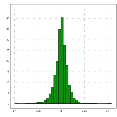
Often the logarithmic returns are studied instead of the deltas. Because of
![]()
the logarithmic returns are approximately the relative changes of the DAX in each period.
>logret:=differences(log(rate)); plot2d(logret,distribution=40):
The rate has a bias, of course, but only a very small one. However, the deviation is quite high, so it is already almost unpredictable.
>mr:=mean(delta), dr:=dev(delta)
0.491942274306
66.4036869492
The same applies to the logarithmic returns.
>mlr:=mean(logret), dlr:=dev(logret)
0.000204901882387
0.0146272945383
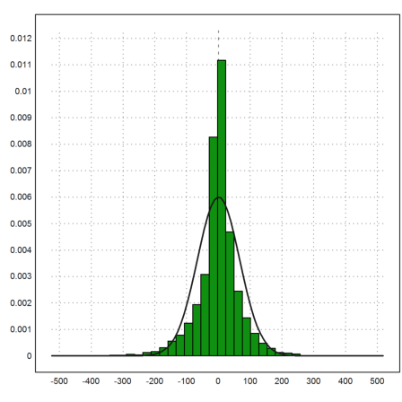
The Gauß normal distribution does not really look like a good fit, and in fact it isn't.
>plot2d(delta,distribution=40);  ...
 plot2d("qnormal(x,mr,dr)",add=1,thickness=2):
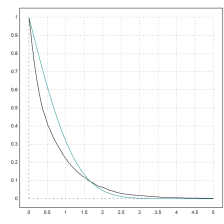
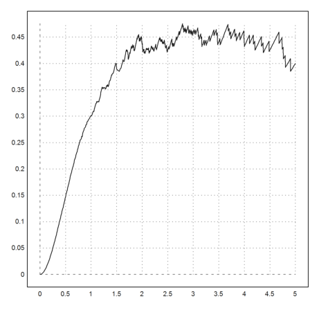
Especially, if we plot the excessive values, we see that there are far more than expected. The function "excess" defined below computes how many deltas are larger than mr+x*vr.
The black curve is the excess of the DAX deltas, and the colored curve would be the excess of a normal distribution.
>function map excess(x) := sum(abs(delta-mr)>x*dr)/cols(delta); ...
 plot2d("excess",0,5); plot2d("(1-normaldis(x))*2",add=1,color=5):
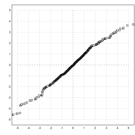
There is another way to study this. We can simply generate a sample of normal distributed values of equal size, sort these values and our deltas, and plot the pairs of data in the plane.
>plot2d(sort(normal(size(delta))*dr+mr),sort(delta), >points,style="."):
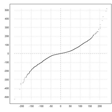
This does not look like a line. So we conclude, that the normal distribution is not a proper model for the deltas of the DAX.
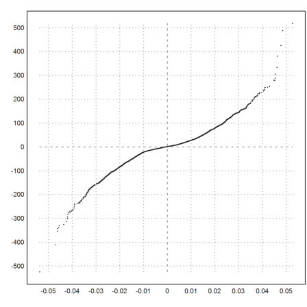
According to the Black-Scholes model, the logarithmic returns of the DAX should be normal distributed.
Let us compute these returns, and plot the distribution.
>plot2d(logret,distribution=40); ...
 plot2d("qnormal(x,mlr,dlr)",thickness=2,>add):

That is not better than what we had before.
>plot2d(sort(normal(size(logret))*dlr+mlr),sort(delta), >points,style="."):
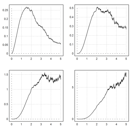
The true behavior is more what Taleb calls a "power law" with exponent 4.
![]()
To see this, we plot the excess times x^a for a=2,3,4,5.
>av=2:6; figure(2,2); ...
 for i=1:4; figure(i); a=av[i]; plot2d("excess(x)*x^a",0,5); end; ...
 figure(0):
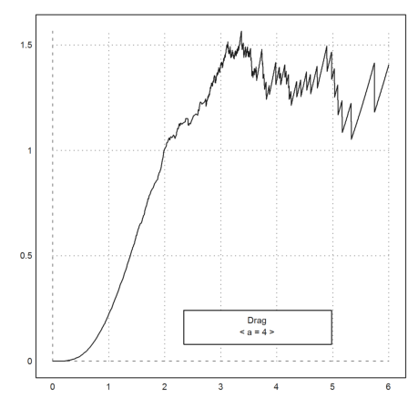
In the following experiment, you can play around with the parameter a. The proper parameter is the one such that
![]()
>function ax (x,a) := excess(x)*x^a; ...
 function plotf (a) := plot2d("ax",0,6;a); ...
 dragvalues("plotf",["a"],4,[1,10],x=0.8,y=0.8,heading="Drag"):
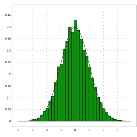
Let us try the same with the normal distribution. The fit is quite well, and there are almost no excessive values, not even in 10000 random values.
>n=10000; sn:=normal(1,n); ...
 plot2d(sn,distribution=40); plot2d("qnormal(x,0,1)",add=1):
The distribution simply does not allow excessive values.
>function map excessn(x) := sum(abs(sn)>x)/n; ...
 plot2d("excessn(x)*x^10",0,6):
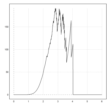
Now the try the same with the "prand" distribution above. It has no variance, so we cannot scale it the same way.
Nevertheless, whatever scaling factor we take, we clearly see the power law with exponent 1.
>n=10000; sn:=prand(1,n); ...
 plot2d("excessn(x*3)*x",0,5):
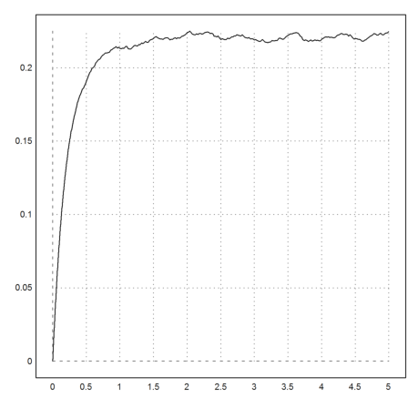
Likewise for the power law 2. Compare this to the normal distribution and the distribution of the DAX!
>n=1000; sn:=p1randr(1,n); plot2d("excessn(x)*x^2",0,5):
We find that the deltas of the DAX obey a power law with exponent 4. This distribution has already a finite variance.
I like to add my personal opinion. From the graph alone, the DAX behaves randomly, and due to the large variance is unpredictable. Only with insider knowledge, combined with knowledge about the general behavior of investors (which may have nothing to do with the real economical development), trends may be predicted and exploited.