by R. Grothmann
In this notebook, we want to do some spherical computations. The functions are contained in the file "spherical.e" in the examples folder.
We need to load that file first.
>load "spherical.e";
To enter a geographical position, we use a vector with two coordinates in radians (north and east, negative values for south and west). The following are the coordinates for the Campus of the Catholic University in Eichstätt.
>EI=[rad(48,53.371),rad(11,11.330)]
[0.853283, 0.195282]
You can print this position with sposprint (spherical position print).
>sposprint(EI)
N 48°53.371' E 11°11.330'
Let us add two more towns, Ingolstadt and Neuburg.
>IN=[rad(48,45.854),rad(11,25.055)]; ND=[rad(48,44.248),rad(11,10.712)];
>sposprint(IN), sposprint(ND),
N 48°45.854' E 11°25.055'
N 48°44.248' E 11°10.712'
First we compute the vector from one to the other on an ideal ball. This vector is [heading,distance] in radians. To compute the distance on the earth, we multiply with the earth radius at a latitude of 48°.
>br=svector(EI,IN); deg(br[1]), br[2]*rearth(48°)->km
129.671788237
21.766496146
This is a good approximation. The following routines use even better approximations. On such a short distance the result is almost the same.
>esdist(EI,IN)->" km"
21.7654976508 km
There is a function for the heading, taking the elliptical shape of the earth into account. Again, we print in an advanced way.
>sdegprint(esdir(EI,IN))
129.67°
The angle of a triangle exceeds 180° on the sphere.
>asum=sangle(IN,EI,ND)+sangle(EI,IN,ND)+sangle(IN,ND,EI); deg(asum)
180.000207484
This can be used to compute the area of the triangle. Note: For small triangles, this is not accurate due to the subtraction error in asum-pi.
>(asum-pi)*rearth(48°)^2->" km^2"
146.771319034 km^2
There is a function for this, which uses the mean latitude of the triangle to compute the earth radius, and takes care of rounding errors for very small triangles.
>esarea(IN,EI,ND)->" km^2"
146.757696278 km^2
We can also add vectors to positions. A vector contains the heading and the distance, both in radians. To get a vector, we use svector. To add a vector to a position, we use saddvector.
>v=svector(EI,IN); sposprint(saddvector(EI,v)), sposprint(IN),
N 48°45.854' E 11°25.055'
N 48°45.854' E 11°25.055'
These functions assume an ideal ball. The same on the earth.
>sposprint(esadd(EI,esdir(EI,IN),esdist(EI,IN))), sposprint(IN),
N 48°45.854' E 11°25.055'
N 48°45.854' E 11°25.055'
Let us turn to a larger example, which I found in the Internet, Brandenburger Tor in Berlin, and the Tejo bridge in Lissabon. For Lissabon, take a negative value for the west coordinate.
>Berlin=[52.5164°,13.3777°]; Lissabon=[38.692668°,-9.177944°];
>sposprint(Berlin), sposprint(Lissabon)
N 52°30.984' E 13°22.662'
N 38°41.560' W 9°10.677'
According to Google Earth, the distance is 2315.75km. We get a good approximation.
>esdist(Lissabon,Berlin)->" km"
2313.67485976 km
The heading is the same as the one computed in Google Earth.
>degprint(esdir(Lissabon,Berlin))
41°3'5.08''
However, we do no longer get the exact target position, if we add the heading and distance to the orginal position. This is so, since we do not compute the inverse function exactly, but take an approximation of the earth radius along the path.
>sposprint(esadd(Berlin,esdir(Berlin,Lissabon),esdist(Berlin,Lissabon)))
N 38°41.557' W 9°10.680'
The error is not large, however.
>sposprint(Lissabon),
N 38°41.560' W 9°10.677'
Of course, we cannot sail with the same heading from one destination to another, if we want to take the shortest path. Imagine, you fly NE starting at any point on the earth. Then you will spiral to the north pole. Great circles do not follow a constant heading!
The following computation shows that we are way off the correct destination, if we use the same heading during our travel.
>dist=esdist(Berlin,Lissabon); hd=esdir(Berlin,Lissabon);
Now we add 10 times one-tenth of the distance, using the heading to Lissabon, we got in Berlin.
>p=Berlin; loop 1 to 10; p=esadd(p,hd,dist/10); end;
The result is far off.
>sposprint(p), skmprint(esdist(p,Lissabon))
N 41°0.566' W 12°5.348'
   357.810km
As another example, let us take two points on the earth at the same lattitude.
>P1=[30°,10°]; P2=[30°,50°];
The shortest path from P1 to P2 is not the circle of lattitude 30°, but a shorter path starting 10° further north at P1.
>sdegprint(esdir(P1,P2))
79.69°
But, if we follow this compass reading, we will spiral to the north pole! So we must adjust our heading along the way. For rough purposes, we adjust it at 1/10 of the total distance.
>p=P1;  dist=esdist(P1,P2); ...
   loop 1 to 10; dir=esdir(p,P2); sdegprint(dir), p=esadd(p,dir,dist/10); end;
     79.69°
     81.67°
     83.71°
     85.78°
     87.89°
     90.00°
     92.12°
     94.22°
     96.29°
     98.33°
The distances are not right, since we will add a bit off error, if we follow the same heading for too long.
>skmprint(esdist(p,P2))
0.203km
We get a good approximation, if we adjust out heading after each 1/100 of the total distance from Berlin to Lissabon.
>p=Berlin; dist=esdist(Berlin,Lissabon); ...
   loop 1 to 100; p=esadd(p,esdir(p,Lissabon),dist/100); end;
>skmprint(esdist(p,Lissabon))
0.057km
For navigational purposes, we can get a sequence of GPS position along the great circle to Lissabon with the function navigate.
>load spherical; v=navigate(Berlin,Lissabon,10); ...
   loop 1 to rows(v); sposprint(v[#]), end;
N 52°30.984' E 13°22.662'
N 51°21.596' E 10°34.058'
N 50°8.382' E 7°53.992'
N 48°51.693' E 5°22.083'
N 47°31.853' E 2°57.902'
N 46°9.158' E 0°40.991'
N 44°43.881' W 1°29.117'
N 43°16.269' W 3°32.890'
N 41°46.547' W 5°30.784'
N 40°14.916' W 7°23.240'
N 38°41.560' W 9°10.677'
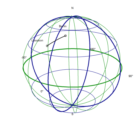
We write a function, which plots the earth, the two positions, and the positions in between.
>function testplot ...
 useglobal;
 plotearth;
 plotpos(Berlin,"Berlin"); plotpos(Lissabon,"Lissabon");
 plotposline(v);
 endfunction
Now plot everything.
>plot3d("testplot",>own,>user,zoom=4):
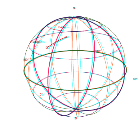
Or use plot3d to get an anaglyph view of it. This looks really great with red/cyan glasses.
>plot3d("testplot",own=1,anaglyph=1,zoom=4):